Other datasets
Up to this moment, we have only shown how the package performs with our
own dataset. The moment of truth is when we test our software with other
people’s datasets. In this section we have compiled saturation
mutagenesis datasets found in the literature and we reproduce the
analysis. Not only does the package works with other datasets, but also
it allows to customize a wide range of parameters such as color maps,
scales, etc. Furthermore, on top of testing the resilience of
mutagenesis_visualization, we are providing extra examples on how to
use this API.
%matplotlib inline
from typing import Dict, Union, List
from pandas.core.frame import DataFrame
import numpy as np
import pandas as pd
import matplotlib as plt
import copy
from mutagenesis_visualization import Screen
from mutagenesis_visualization import load_demo_datasets
from mutagenesis_visualization import DemoObjects
from mutagenesis_visualization.main.utils.data_paths import PDB_1ERM, PDB_1A5R, PDB_1ND4
DEMO_DATASETS: Dict[str, Union[np.array, DataFrame]] = load_demo_datasets()
- Function reviewed in this section:
Load objects
For simplicity, we also have added the option of loading those datasets into objects automatically There are 10 objects to load from other papers (hras_rbd, hras_gapgef, bla_obj, sumo_obj, mapk1_obj, ube2i_obj, tat_obj, rev_obj, asynuclein_obj, aph_obj, b11l5f_obj) and all the heatmaps from the Hidalgo et al. eLife 2022 paper (hras_166_gap, hras_166_rbd, hras_188_baf3, hras_180_gap, hras_180_rbd, kras_165_gap, kras_165_gapgef, kras_173_gapgef, kras_165_gef, kras_173_gef, kras_165_rbd, kras_173_gap, kras_173_rbd, hras_166_gapgef, krasq61l_173_gap, and krasq61l_173_rbd.).
Hidalgo et al. eLife 2022 paper
The figures of the Hidalgo et al. eLife 2022 paper were created using
mutagenesis-visualization. To retrieve the objects, just instantiate the
class DemoObjects and then access each of the datasets.
# instantiate
demo_objects = DemoObjects()
# access the datasets
demo_objects.hras_188_baf3.heatmap()
Beta Lactamase
Create object
#https://www.uniprot.org/uniprot/P62593#sequences
# Order of amino acid substitutions in the hras_enrichment dataset
aminoacids: List[str] = list(DEMO_DATASETS['df_bla'].index)
neworder_aminoacids: List[str] = list('DEKHRGNQASTPCVYMILFW')
# First residue of the hras_enrichment dataset. Because 1-Met was not mutated, the dataset starts at residue 2
start_position = DEMO_DATASETS['df_bla'].columns[0]
# Define sequence. If you dont know the start of the sequence, just add X's
sequence_bla_x = 'MSIQHFRVALIPFFAAFCLPVFAHPETLVKVKDAEDQLGARVGYIELDLNSGKILESFRP' + 'EERFPMMSTFKVLLCGAVLSRVDAGQEQLGRRIHYSQNDLVEYSPVTEKHLTDGMTVREL' + 'CSAAITMSDNTAANLLLTTIGGPKELTAFLHNMGDHVTRLDRWEPELNEAIPNDERDTTM' + 'PAAMATTLRKLLTGELLTLASRQQLIDWMEADKVAGPLLRSALPAGWFIADKSGAGERGS' + 'RGIIAALGPDGKPSRIVVIYTTGSQATMDERNRQIAEIGASLIKHW'
# Define secondary structure
secondary_bla = [['L0'] * 23, ['α1'] * (38 - 23), ['L1'] * 2, ['β1'] * (48 - 40),
['L2'] * 5, ['β2'] * (57 - 53), ['L3'] * (68 - 57), ['α2'] * (84 - 68),
['L4'] * (95 - 84), ['α3'] * (100 - 95), ['L5'] * (103 - 100),
['α4'] * (110 - 103), ['L6'] * (116 - 110), ['α5'] * (140 - 116),
['L7'] * (1), ['α6'] * (153 - 141), ['L8'] * (164 - 153),
['α7'] * (169 - 164), ['L9'] * (179 - 169), ['α8'] * (194 - 179), ['L10'] *
3, ['α9'] * (210 - 197), ['L11'] * (227 - 210), ['β3'] * (235 - 227),
['L12'] * (240 - 235), ['β4'] * (249 - 240), ['L13'] * (254 - 249),
['β5'] * (262 - 254), ['L14'] * (266 - 262), ['α10'] * (286 - 266)]
bla_obj: Screen = Screen(
DEMO_DATASETS['df_bla'], sequence_bla_x, aminoacids, start_position, 0, secondary_bla
)
2D Plots
# Create full heatmap
bla_obj.heatmap(
colorbar_scale=(-3, 3),
neworder_aminoacids=neworder_aminoacids,
title='Beta Lactamase',
show_cartoon=True,
)
# Miniheatmap
bla_obj.miniheatmap(
title='Wt residue Beta Lactamase',
neworder_aminoacids=neworder_aminoacids,
)
# Positional mean
bla_obj.enrichment_bar(
figsize=[10, 2.5],
mode='mean',
show_cartoon=True,
yscale=[-3, 0.25],
title='',
)
# Kernel
bla_obj.kernel(
histogram=True, title='Beta Lactamase', xscale=[-4, 1]
)
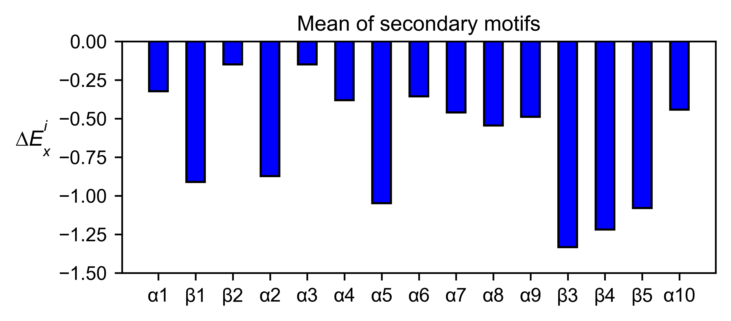
# Graph bar of the mean of each secondary motif
bla_obj.secondary_mean(
yscale=[-1.5, 0],
figsize=[5, 2],
title='Mean of secondary motifs',
)
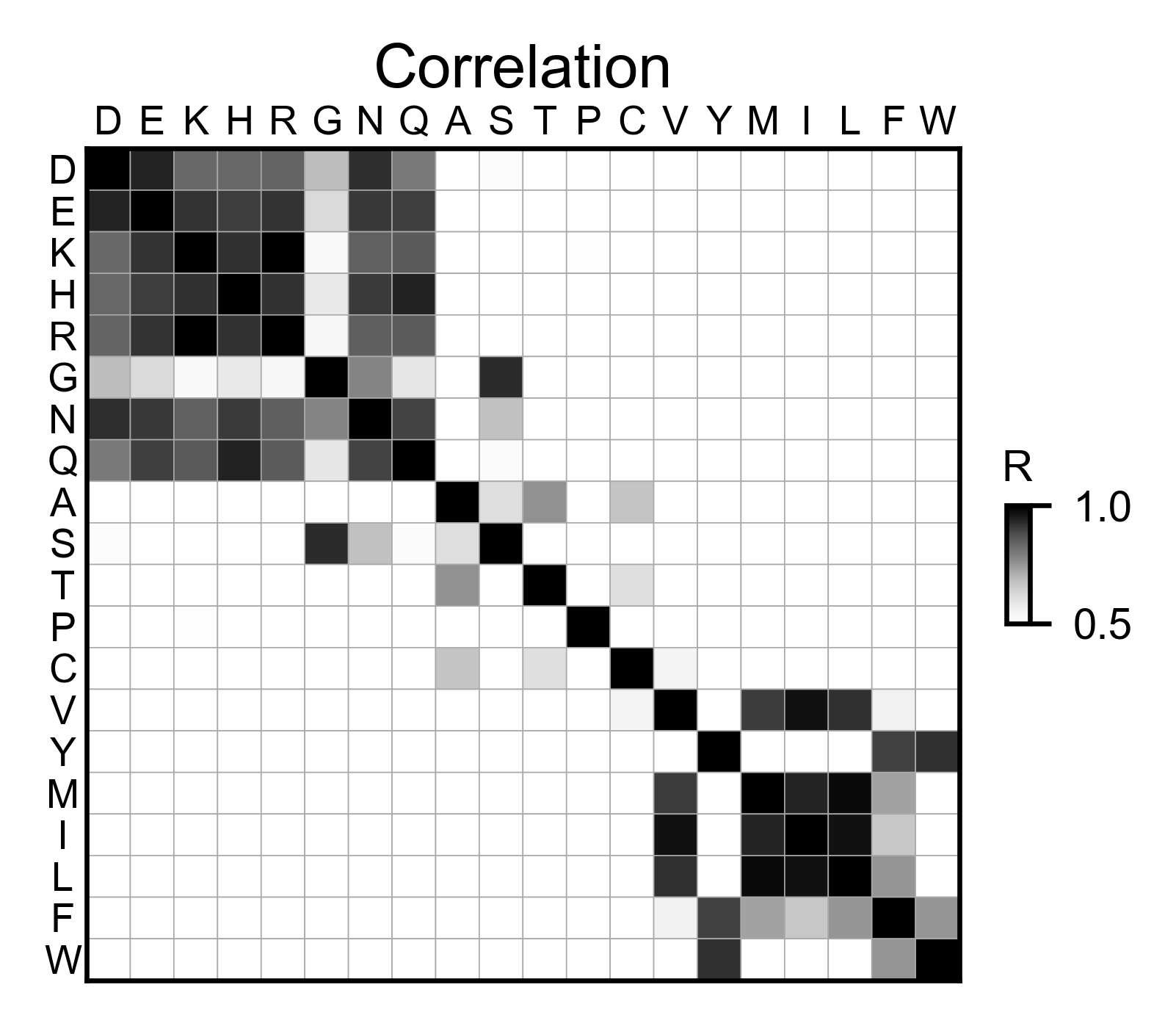
# Correlation between amino acids
bla_obj.correlation(
colorbar_scale=[0.5, 1],
title='Correlation',
neworder_aminoacids=neworder_aminoacids,
)
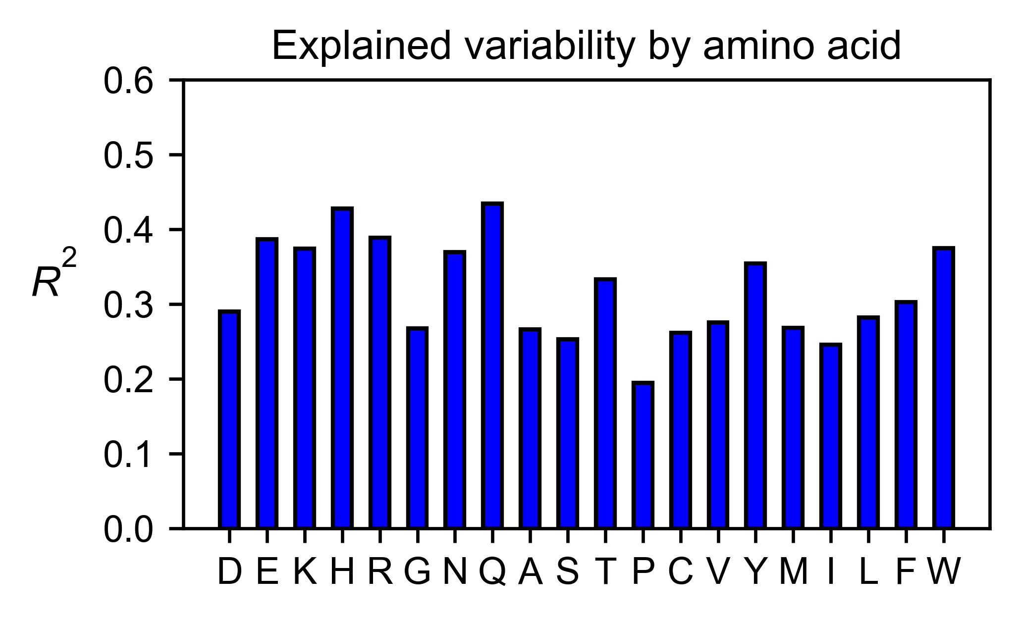
# Explained variability by amino acid
bla_obj.individual_correlation(
yscale=[0, 0.6],
title='Explained variability by amino acid',
)
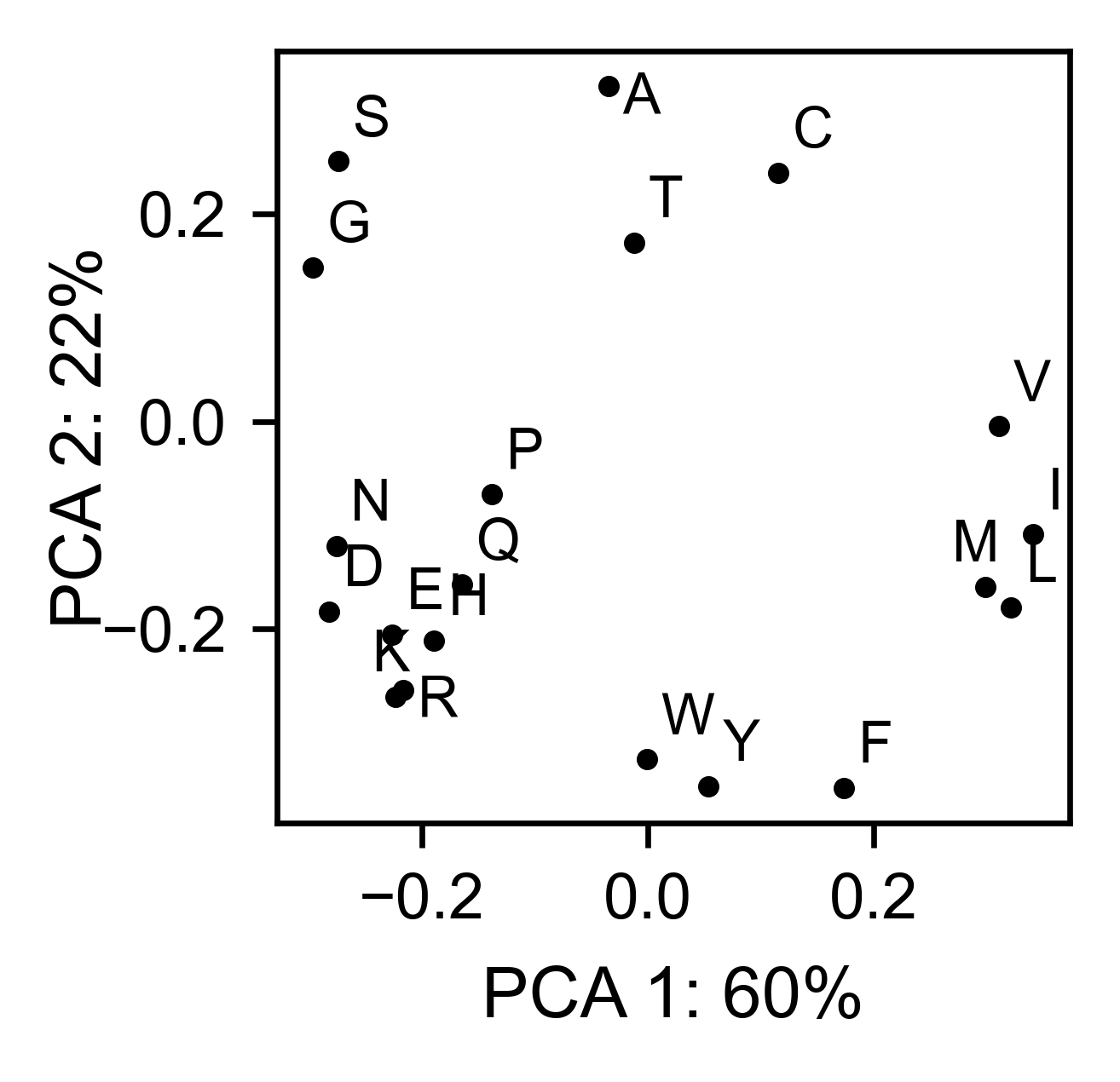
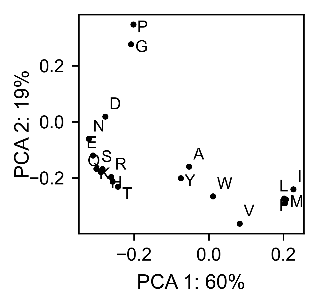
# PCA by amino acid substitution
bla_obj.pca(
title='',
dimensions=[0, 1],
figsize=(2, 2),
adjustlabels=True,
)
# PCA by secondary structure motif
bla_obj.pca(
title='',
mode='secondary',
dimensions=[0, 1],
figsize=(2, 2),
adjustlabels=True,
)
3D Plots
# Plot 3-D plot
bla_obj.plotly_scatter_3d(
mode='mean',
pdb_path=PDB_1ERM,
position_correction=2,
title='Scatter 3D',
squared=False,
x_label='x',
y_label='y',
z_label='z',
)
# Plot 3-D of distance to center of protein, SASA and B-factor
bla_obj.plotly_scatter_3d_pdbprop(
plot=['Distance', 'SASA', 'log B-factor'],
position_correction=2,
pdb_path=PDB_1ERM,
title='Scatter 3D - PDB properties',
)
# Start pymol and color residues. Cut offs are set with gof and lof parameters.
bla_obj.pymol(
pdb=PDB_1ERM, mode='mean', gof=0.2, lof=-1, position_correction=2
)
Sumo1
Create object
#https://doi.org/10.15252/msb.20177908
# Order of amino acid substitutions in the hras_enrichment dataset
aminoacids = list(DEMO_DATASETS['df_sumo1'].index)
# First residue of the hras_enrichment dataset. Because 1-Met was not mutated, the dataset starts at residue 2
start_position = DEMO_DATASETS['df_sumo1'].columns[0]
# Full sequence
sequence_sumo1 = 'MSDQEAKPSTEDLGDKKEGEYIKLKVIGQDSSEIHFKVKMTTHLKKLKESYCQRQGVPMN' + 'SLRFLFEGQRIADNHTPKELGMEEEDVIEVYQEQTGGHSTV'
# Define secondary structure
secondary_sumo1 = [['L0'] * (20), ['β1'] * (28 - 20), ['L1'] * 3, ['β2'] * (39 - 31),
['L2'] * 4, ['α1'] * (55 - 43),
['L3'] * (6), ['β3'] * (65 - 61), ['L4'] * (75 - 65), ['α2'] * (80 - 75),
['L5'] * (85 - 80), ['β4'] * (92 - 85), ['L6'] * (101 - 92)]
sumo_obj: Screen = Screen(
DEMO_DATASETS['df_sumo1'], sequence_sumo1, aminoacids, start_position, 1,
secondary_sumo1
)
2D Plots
# You can use your own colormap or import it from matplotlib
colormap = copy.copy((plt.cm.get_cmap('Blues_r')))
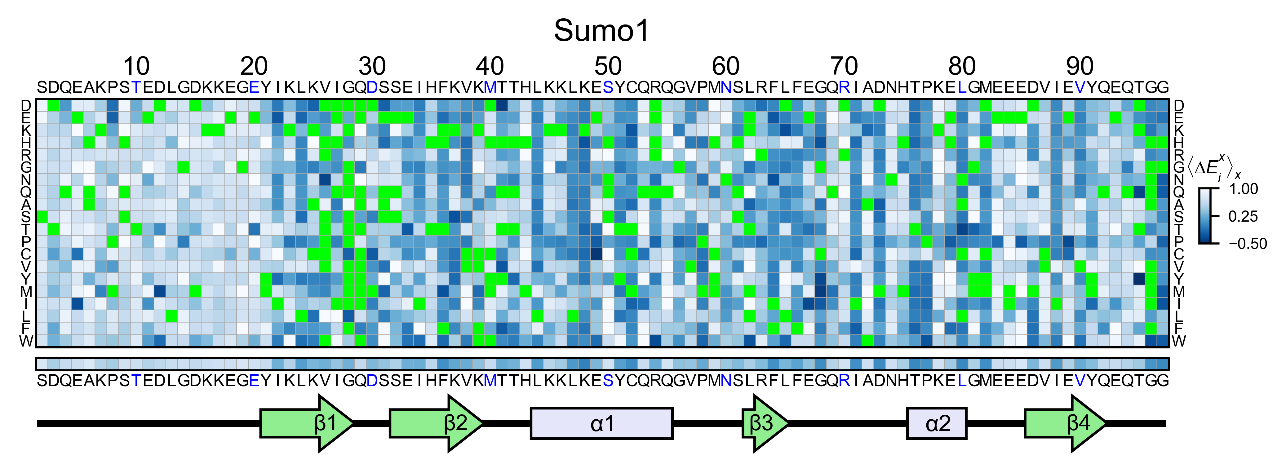
# Create full heatmap
sumo_obj.heatmap(
colorbar_scale=(-0.5, 1),
neworder_aminoacids=neworder_aminoacids,
title='Sumo1',
colormap=colormap,
show_cartoon=True,
)
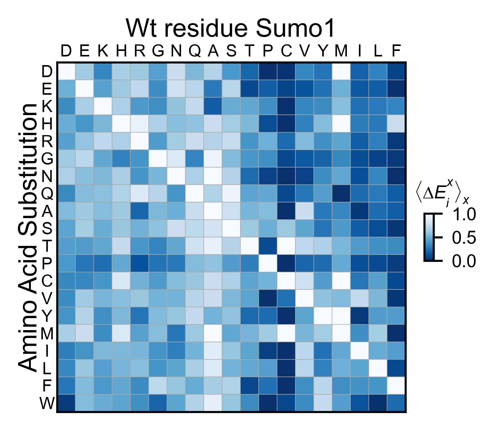
# Miniheatmap
sumo_obj.miniheatmap(
colorbar_scale=(0, 1),
title='Wt residue Sumo1',
neworder_aminoacids=neworder_aminoacids,
colormap=colormap,
)
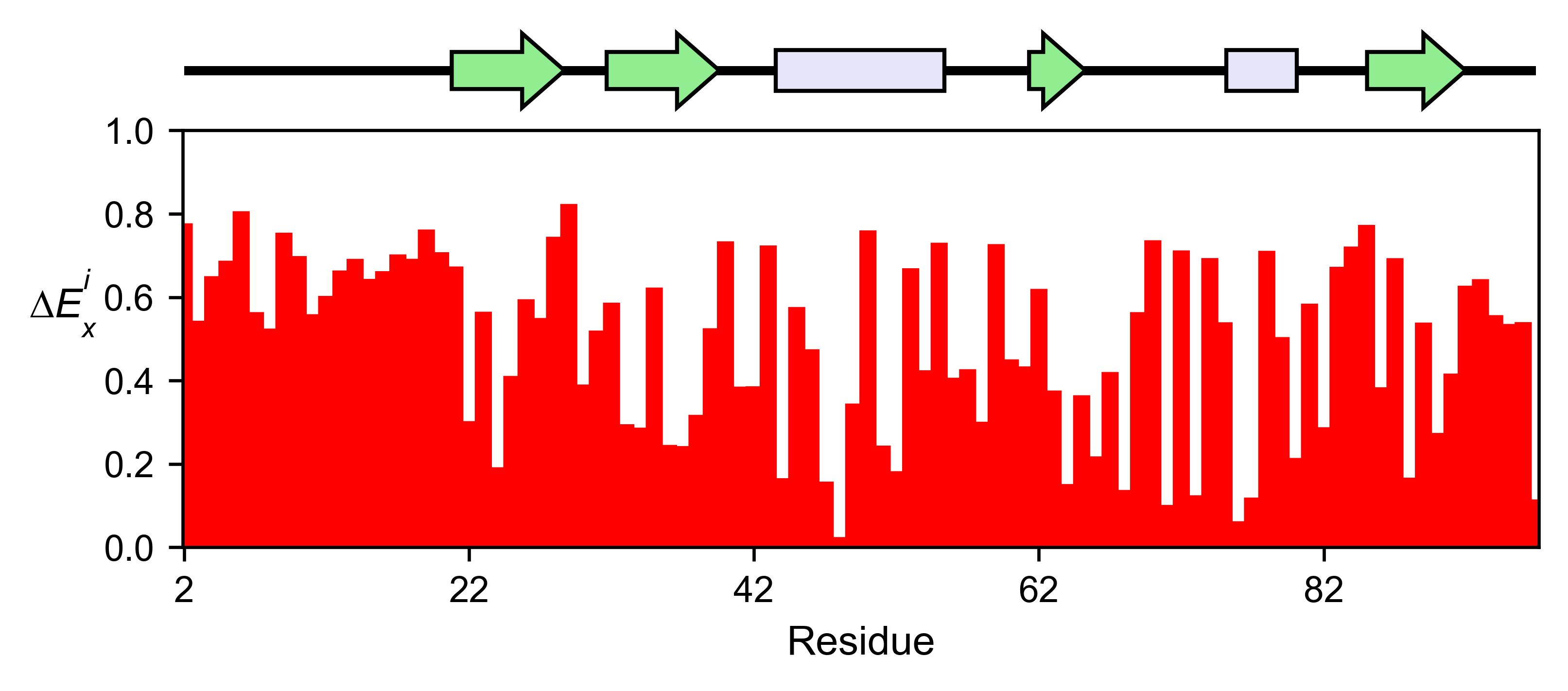
# Positional mean
sumo_obj.enrichment_bar(
figsize=[6, 2.5],
mode='mean',
show_cartoon=True,
yscale=[0, 1],
title='',
)
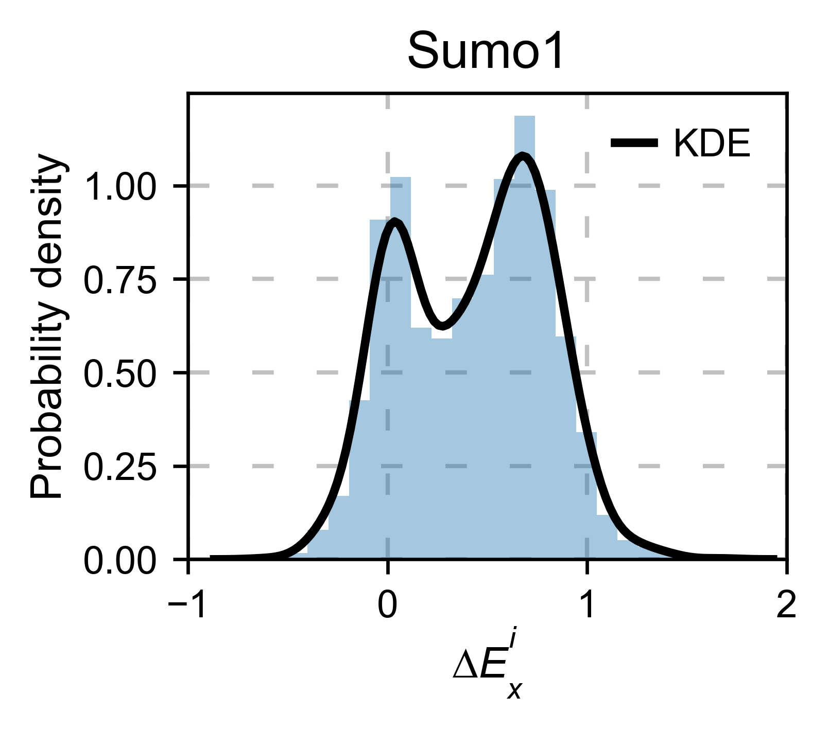
# Kernel
sumo_obj.kernel(histogram=True, title='Sumo1', xscale=[-1, 2], output_file=None)
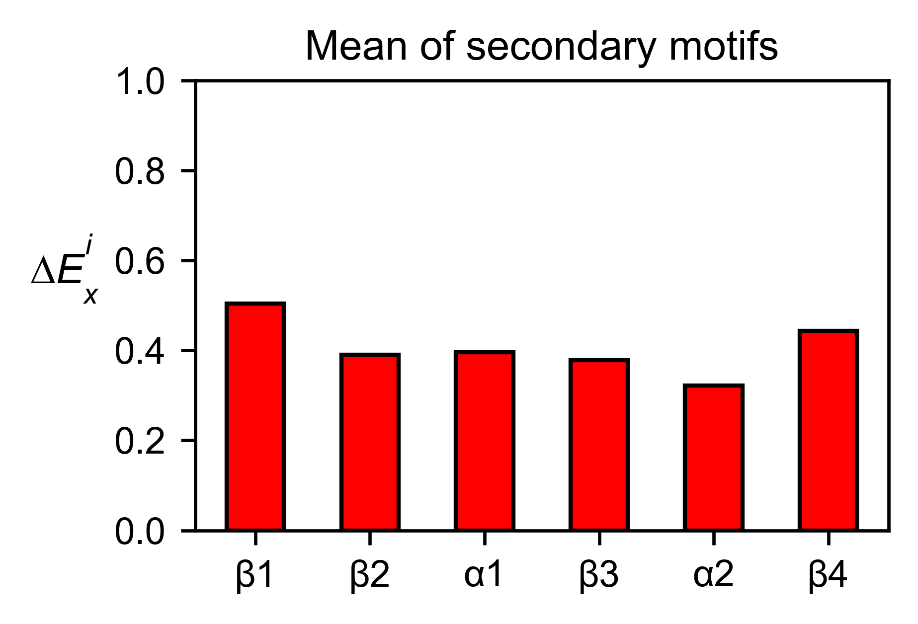
# Graph bar of the mean of each secondary motif
sumo_obj.secondary_mean(
yscale=[0, 1],
figsize=[2, 2],
title='Mean of secondary motifs',
)
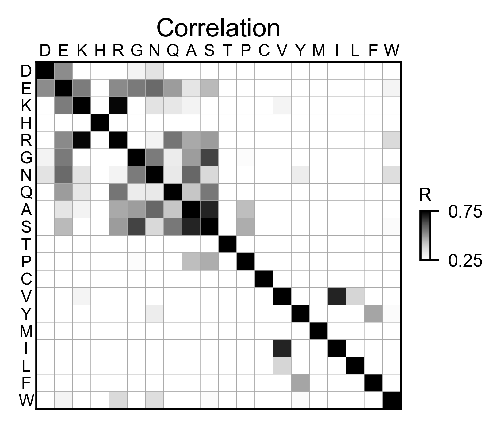
# Correlation between amino acids
sumo_obj.correlation(
colorbar_scale=[0.25, 0.75],
title='Correlation',
neworder_aminoacids=neworder_aminoacids,
)
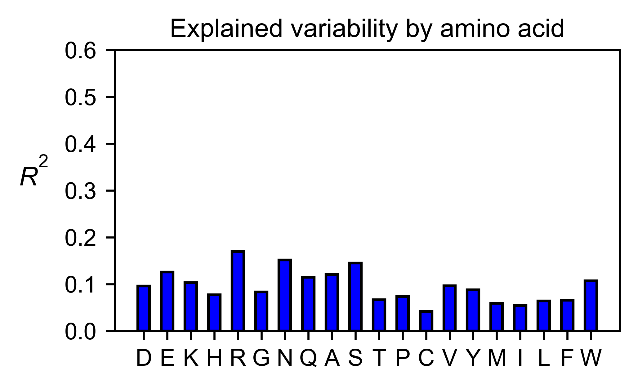
# Explained variability by amino acid
sumo_obj.individual_correlation(
yscale=[0, 0.6],
title='Explained variability by amino acid',
)
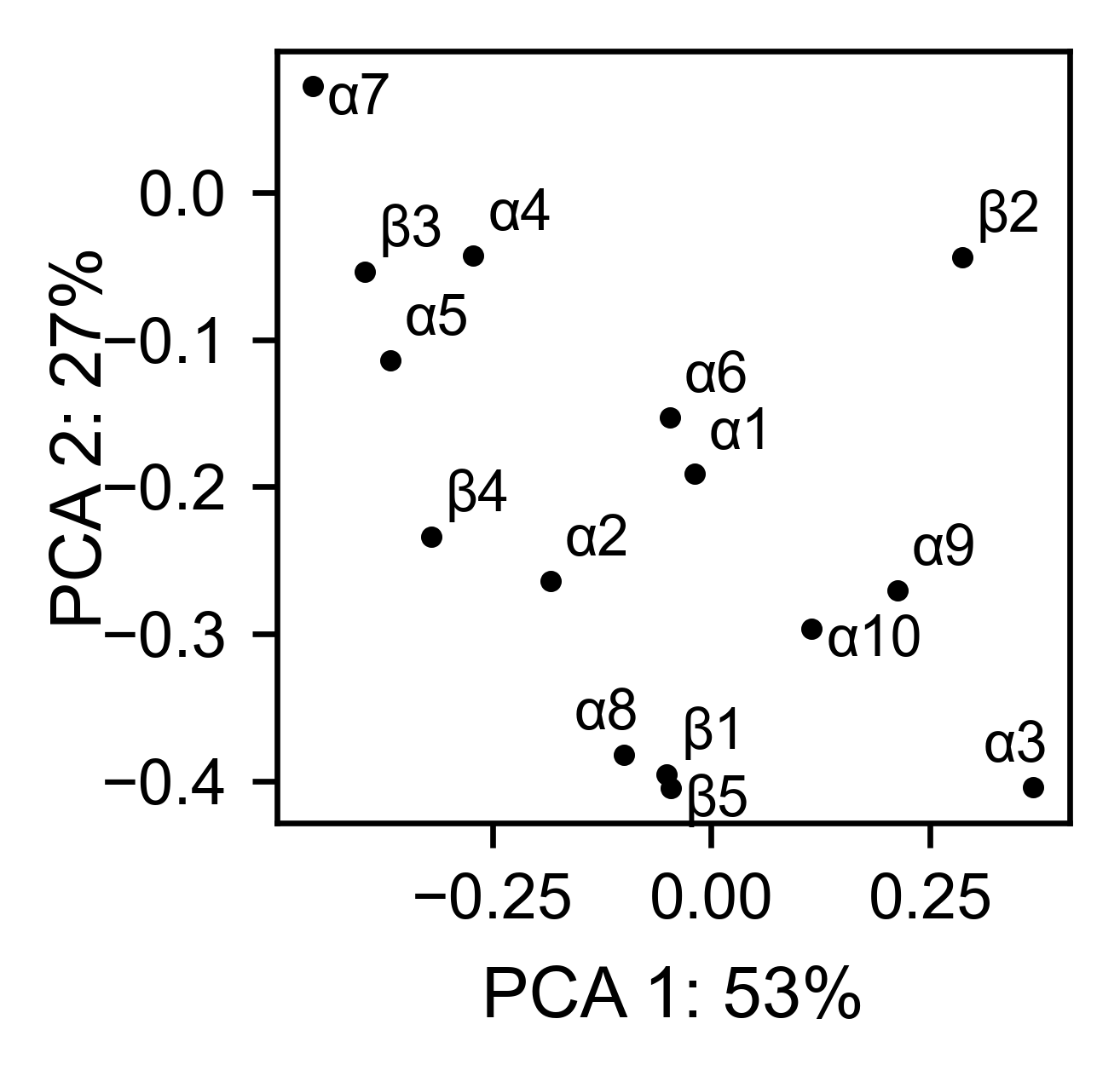
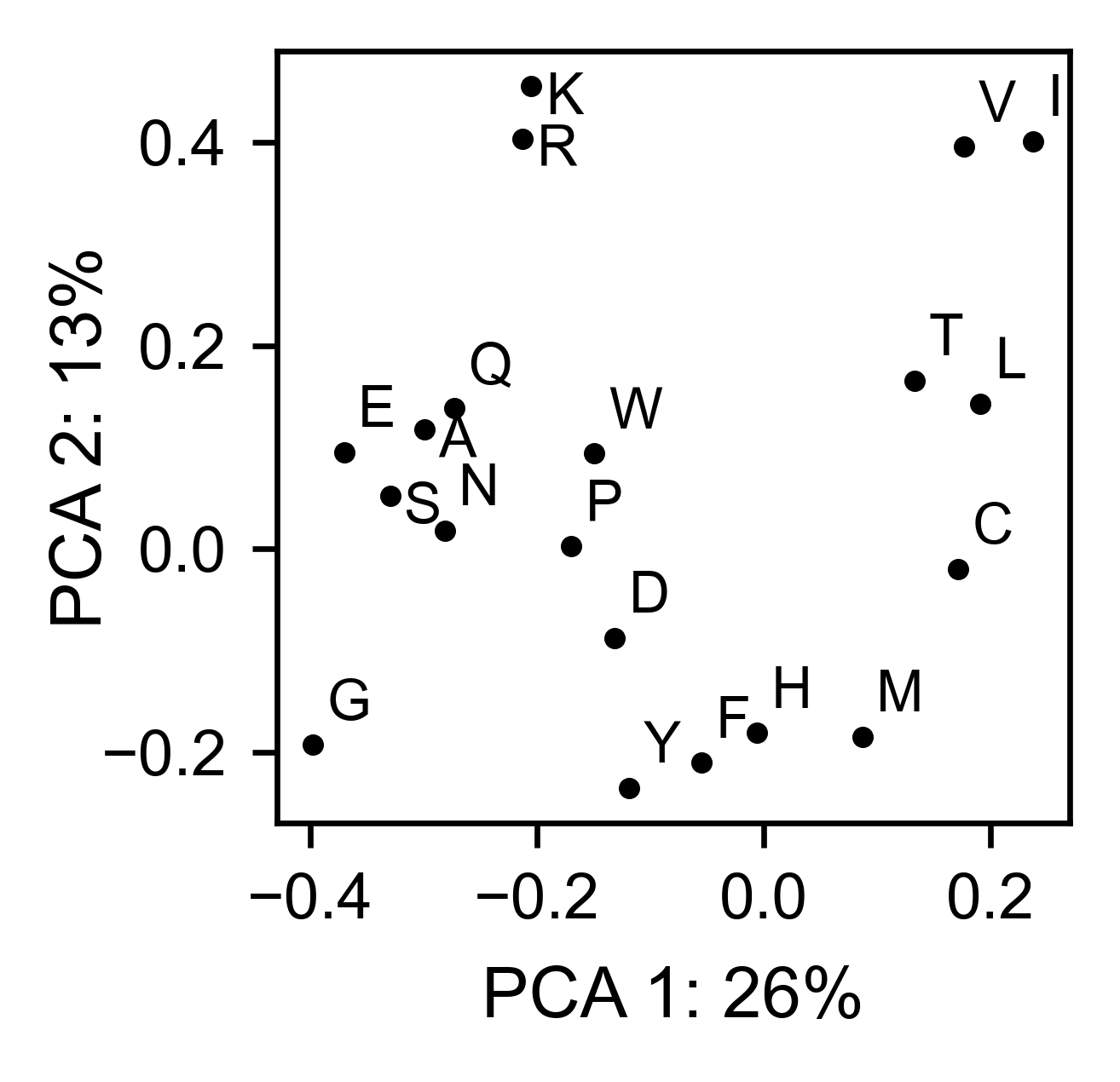
# PCA by amino acid substitution
sumo_obj.pca(
title='',
dimensions=[0, 1],
figsize=(2, 2),
adjustlabels=True,
)
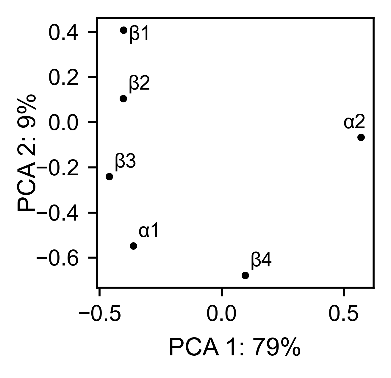
# PCA by secondary structure motif
sumo_obj.pca(
title='',
mode='secondary',
dimensions=[0, 1],
figsize=(2, 2),
adjustlabels=True,
)
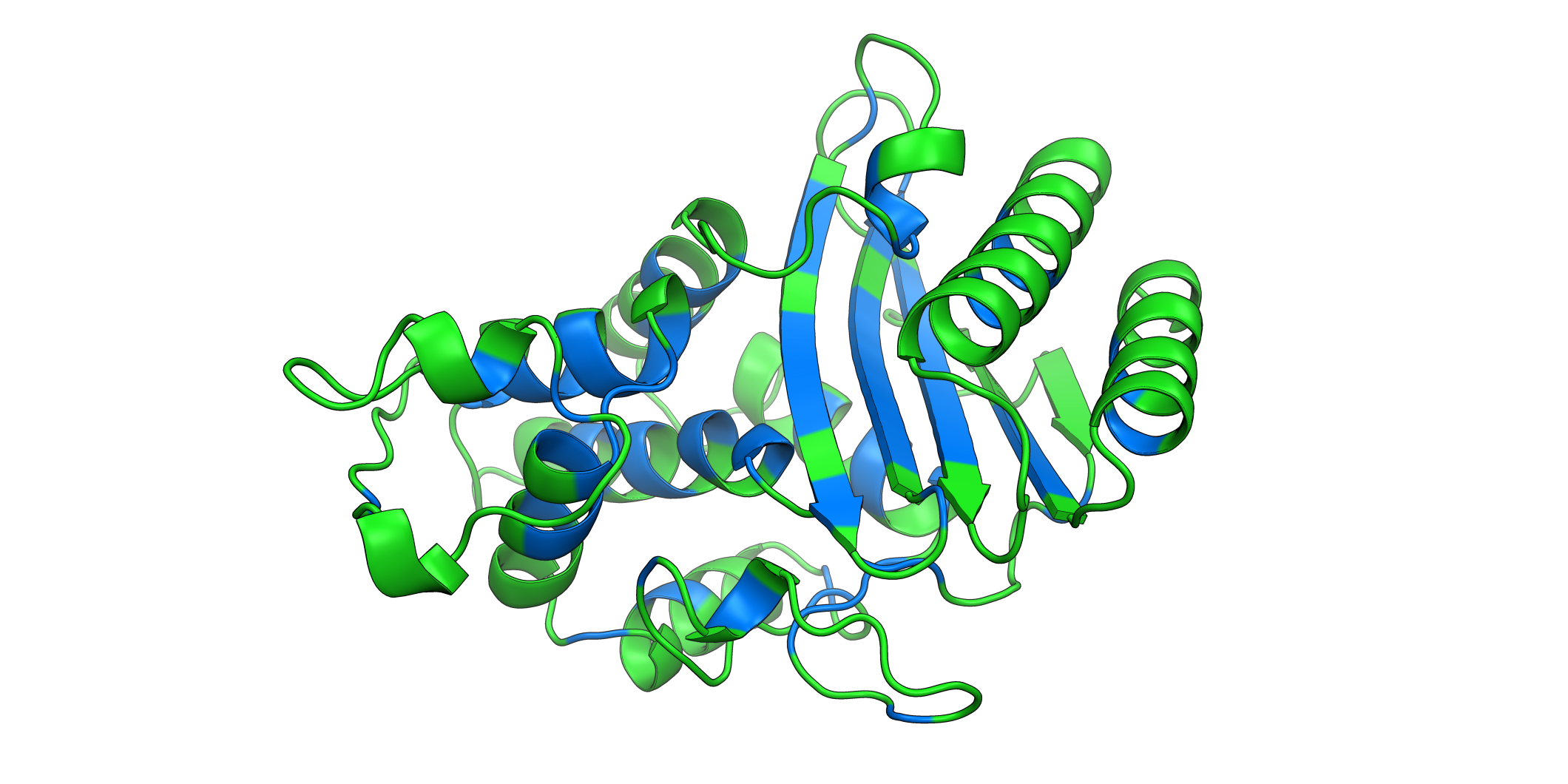
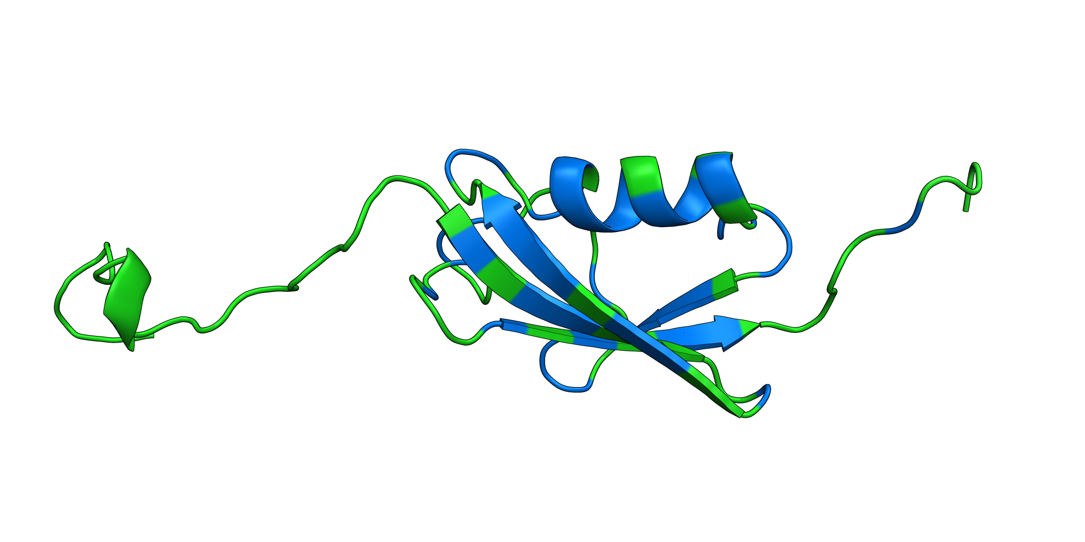
# Open pymol and color the sumo structure
sumo_obj.pymol(pdb=PDB_1A5R, mode='mean', gof=1, lof=0.5)
MAPK1
Create object
# Order of amino acid substitutions in the hras_enrichment dataset
aminoacids = list(DEMO_DATASETS['df_mapk1'].index)
# First residue of the hras_enrichment dataset. Because 1-Met was not mutated, the dataset starts at residue 2
start_position = DEMO_DATASETS['df_mapk1'].columns[0]
# Full sequence
sequence_mapk1_x = 'MAAAAAAGAGPEMVRGQVFDVGPRYTNLSYIGEGAYGMVCSAYDNVNKVRVAIK' + 'KISPFEHQTYCQRTLREIKILLRFRHENIIGINDIIRAPTIEQMKDVYIVQDLMETDLYKLLKTQ' + 'HLSNDHICYFLYQILRGLKYIHSANVLHRDLKPSNLLLNTTCDLKICDFGLARVADPDHDHTGFL' + 'TEYVATRWYRAPEIMLNSKGYTKSIDIWSVGCILAEMLSNRPIFPGKHYLDQLNHILGILGSPSQ' + 'EDLNCIINLKARNYLLSLPHKNKVPWNRLFPNADSKALDLLDKMLTFNPHKRIEVEQALAHPYLE' + 'QYYDPSDEPIAEAPFKFDMELDDLPKEKLKELIFEETARFQPGYRS'
# Create objects
mapk1_obj: Screen = Screen(DEMO_DATASETS['df_mapk1'], sequence_mapk1_x, aminoacids, start_position, 0)
2D Plots
# Create full heatmap
mapk1_obj.heatmap(
colorbar_scale=(-2, 2),
neworder_aminoacids=neworder_aminoacids,
title='MAPK1',
show_cartoon=False,
)
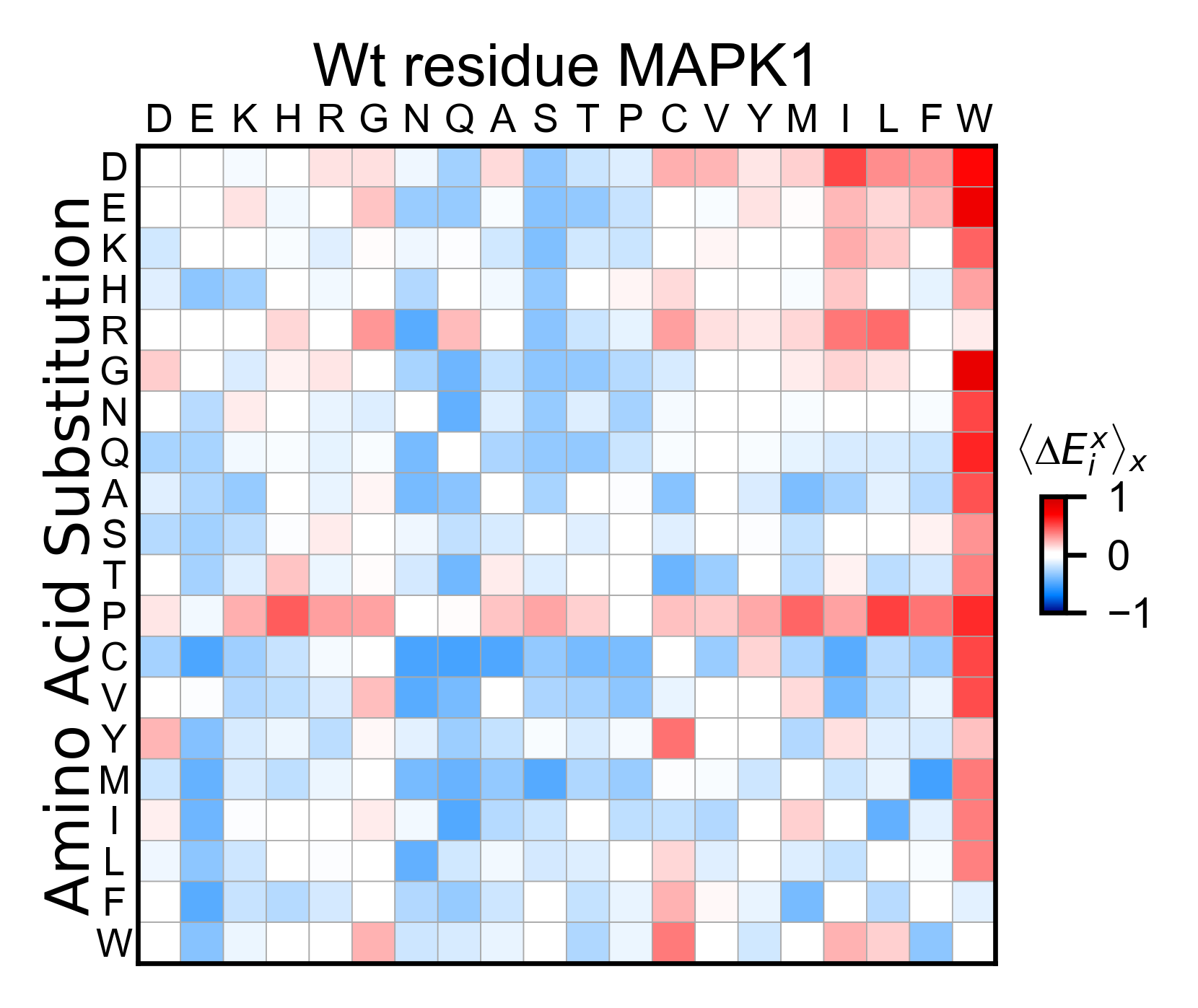
# Miniheatmap
mapk1_obj.miniheatmap(
title='Wt residue MAPK1',
neworder_aminoacids=neworder_aminoacids,
)
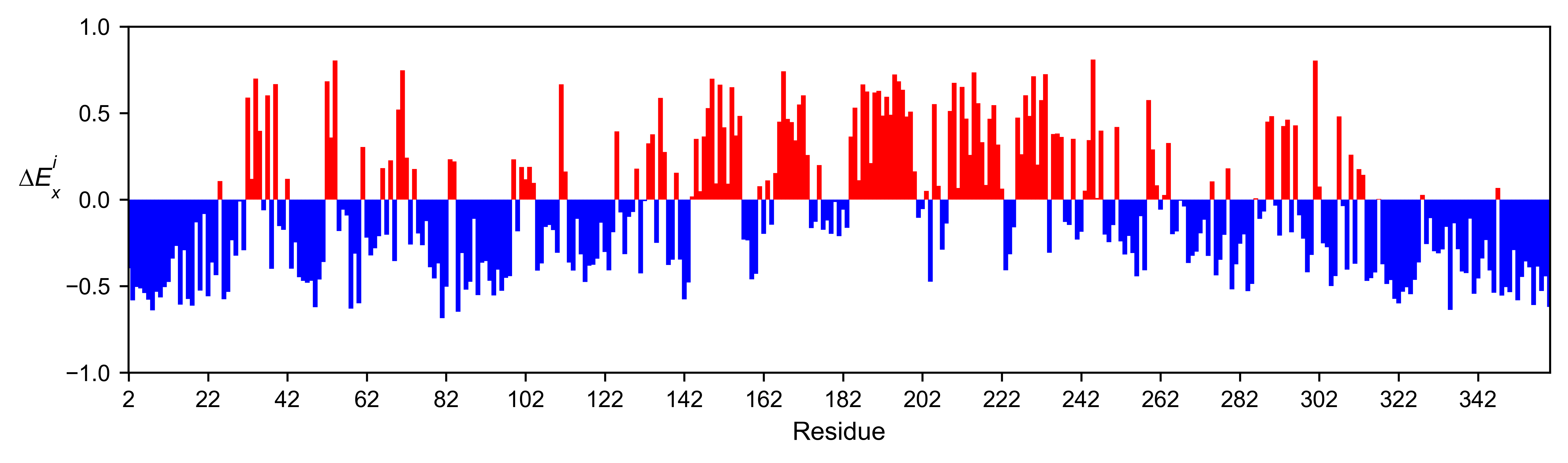
# Positional mean
mapk1_obj.enrichment_bar(
figsize=[10, 2.5],
mode='mean',
show_cartoon=False,
yscale=[-1, 1],
title='',
)
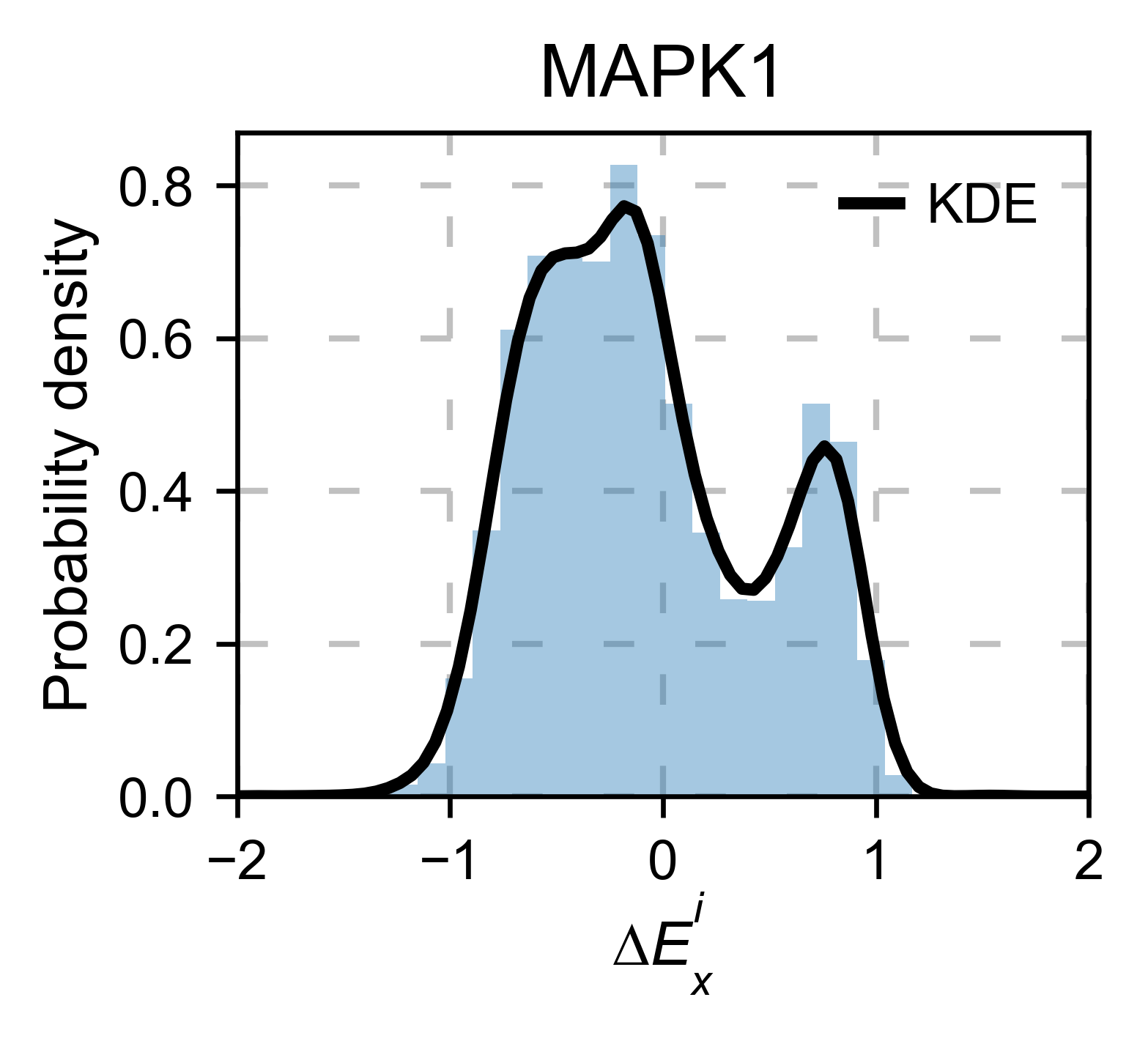
# Kernel
mapk1_obj.kernel(
histogram=True, title='MAPK1', xscale=[-2, 2], output_file=None
)
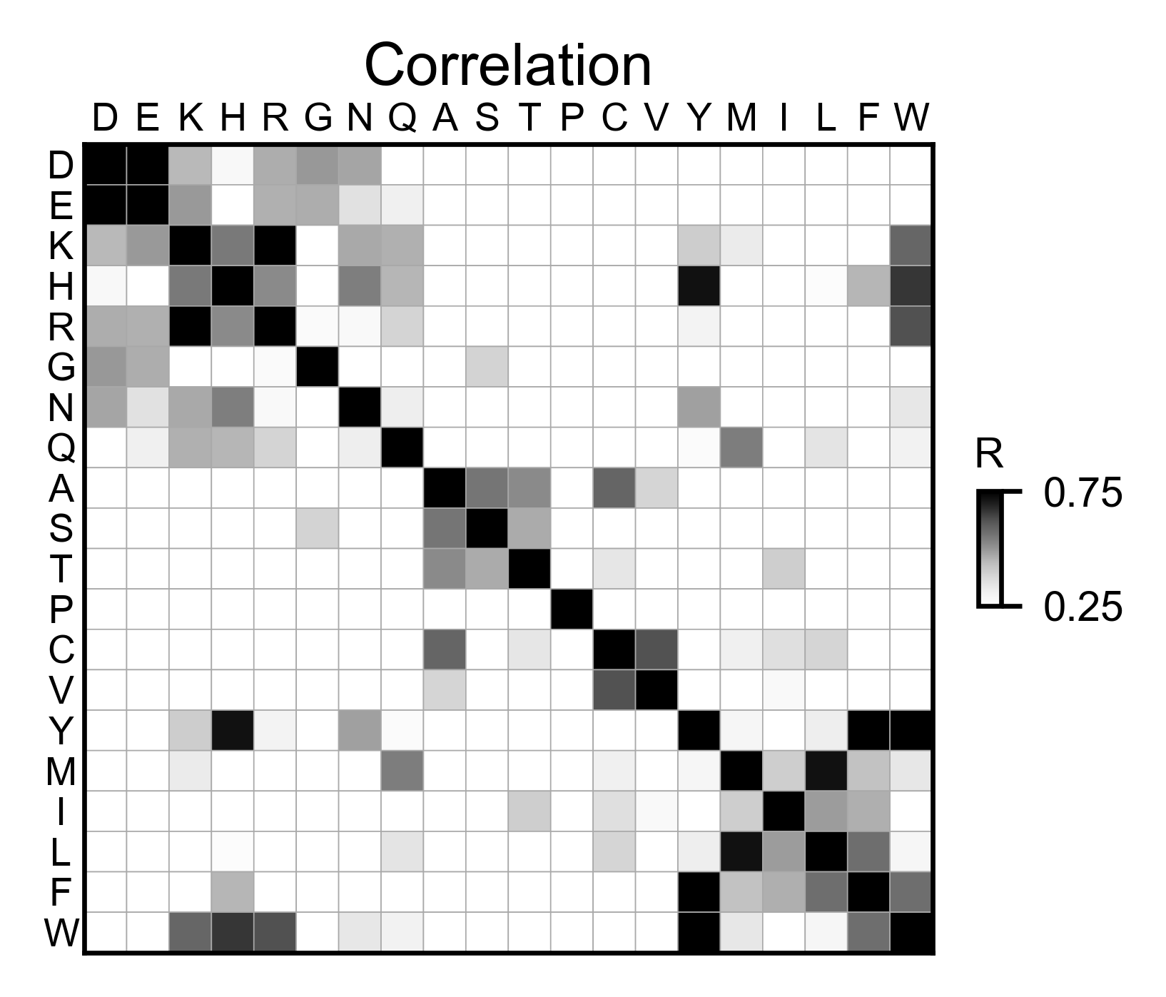
# Correlation between amino acids
mapk1_obj.correlation(
colorbar_scale=[0.25, 0.75],
title='Correlation',
neworder_aminoacids=neworder_aminoacids,
)
# Explained variability by amino acid
mapk1_obj.individual_correlation(
yscale=[0, 0.6],
title='Explained variability by amino acid',
)
# PCA by amino acid substitution
mapk1_obj.pca(
title='',
dimensions=[0, 1],
figsize=(2, 2),
adjustlabels=True,
)

UBE2I
Create object
# Order of amino acid substitutions in the hras_enrichment dataset
aminoacids = list(DEMO_DATASETS['df_ube2i'].index)
# First residue of the hras_enrichment dataset. Because 1-Met was not mutated, the dataset starts at residue 2
start_position = DEMO_DATASETS['df_ube2i'].columns[0]
# Full sequence
sequence_ube2i_x = 'MSGIALSRLAQERKAWRKDHPFGFVAVPTKNPDGTMNLMNWECAIPGKKGTP' + 'WEGGLFKLRMLFKDDYPSSPPKCKFEPPLFHPNVYPSGTVCLSILEEDKDWRPAITIKQ' + 'ILLGIQELLNEPNIQDPAQAEAYTIYCQNRVEYEKRVRAQAKKFAPS'
# Define secondary structure
secondary_ube2i = [['α1'] * (20 - 1), ['L1'] * (24 - 20), ['β1'] * (30 - 24), ['L2'] * 5,
['β2'] * (46 - 35), ['L3'] * (56 - 46), ['β3'] * (63 - 56),
['L4'] * (73 - 63), ['β4'] * (77 - 73), ['L5'] * (93 - 77),
['α2'] * (98 - 93), ['L6'] * (107 - 98), ['α3'] * (122 - 107),
['L7'] * (129 - 122), ['α4'] * (155 - 129), ['L8'] * (160 - 155)]
# Create objects
ube2i_obj: Screen = Screen(
DEMO_DATASETS['df_ube2i'], sequence_ube2i_x, aminoacids, start_position, 1,
secondary_ube2i
)
2D Plots
colormap = copy.copy((plt.cm.get_cmap('Blues_r')))
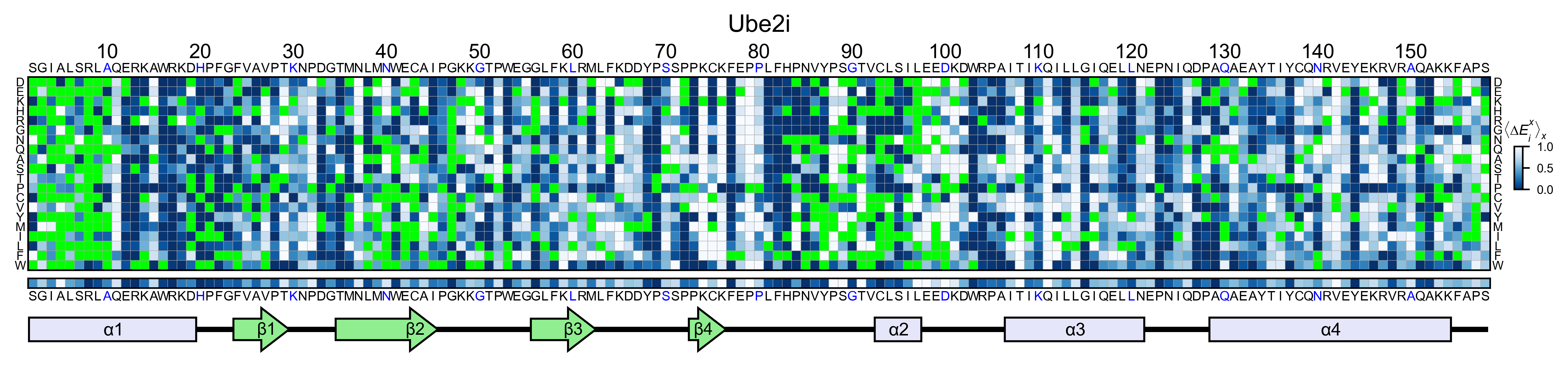
# Create full heatmap
ube2i_obj.heatmap(
colorbar_scale=(0, 1),
neworder_aminoacids=neworder_aminoacids,
title='Ube2i',
colormap=colormap,
show_cartoon=True,
)
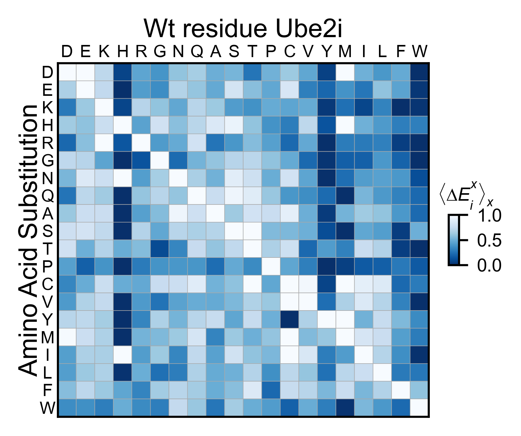
# Miniheatmap
ube2i_obj.miniheatmap(
colorbar_scale=(0, 1),
title='Wt residue Ube2i',
neworder_aminoacids=neworder_aminoacids,
colormap=colormap,
)
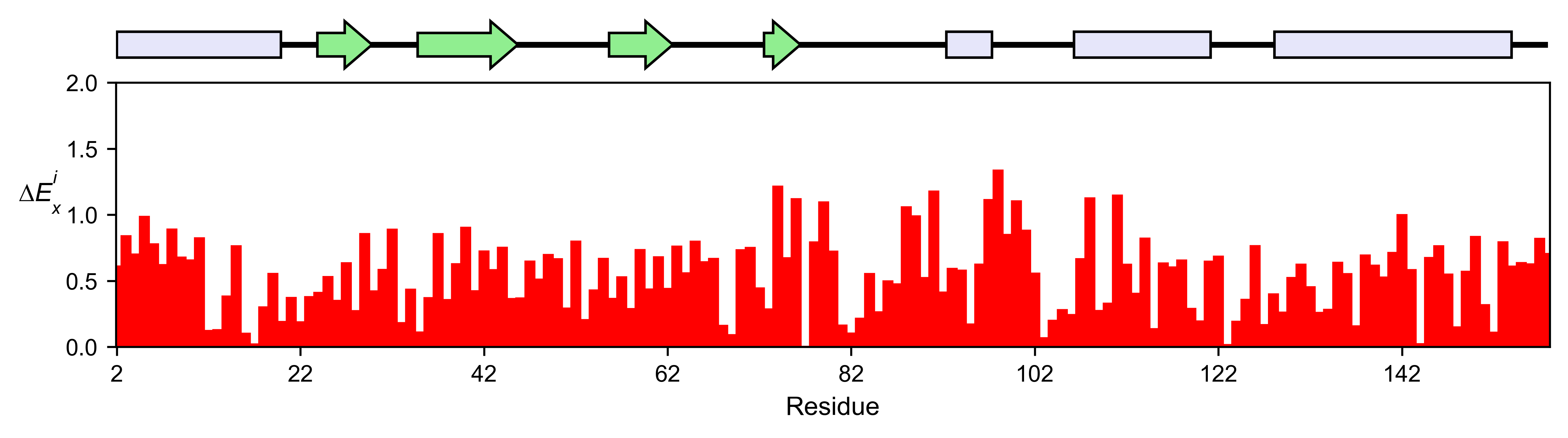
# Positional mean
ube2i_obj.enrichment_bar(
figsize=[10, 2.5],
mode='mean',
show_cartoon=True,
yscale=[0, 2],
title='',
)
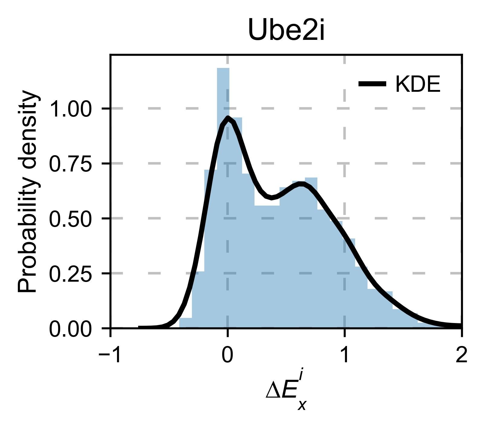
# Kernel
ube2i_obj.kernel(
histogram=True, title='Ube2i', xscale=[-1, 2], output_file=None
)
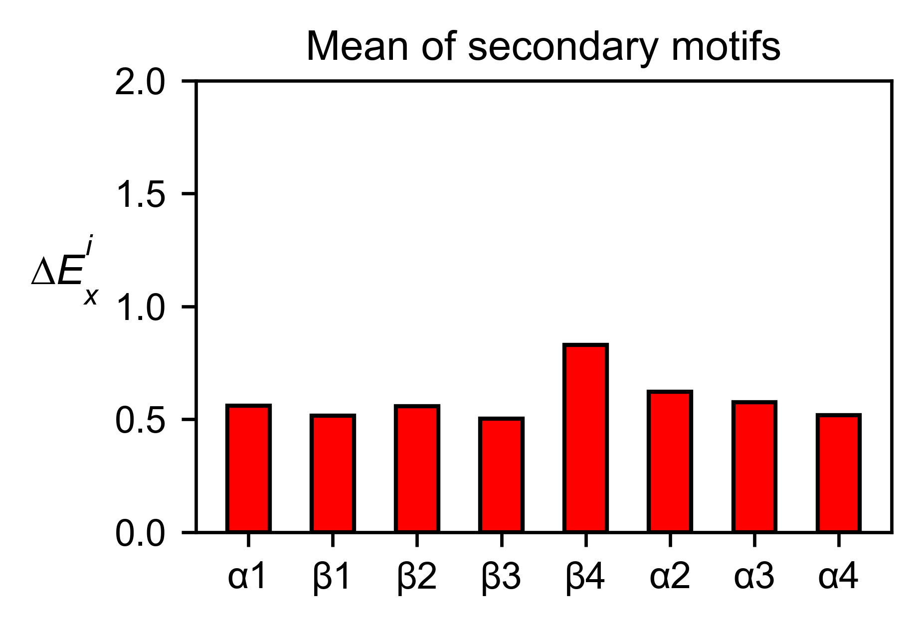
# Graph bar of the mean of each secondary motif
ube2i_obj.secondary_mean(
yscale=[0, 2],
figsize=[3, 2],
title='Mean of secondary motifs',
)
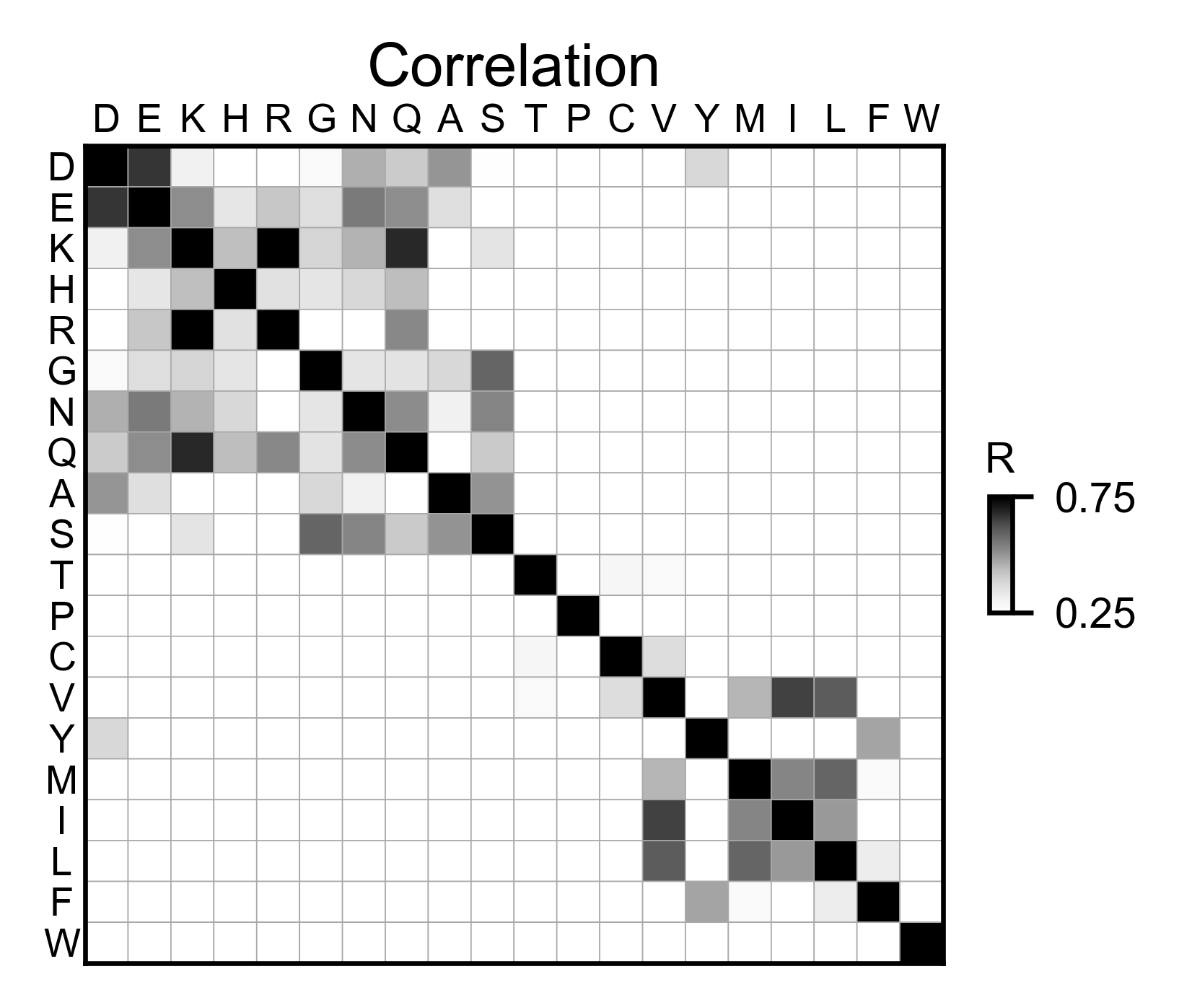
# Correlation between amino acids
ube2i_obj.correlation(
colorbar_scale=[0.25, 0.75],
title='Correlation',
neworder_aminoacids=neworder_aminoacids,
)
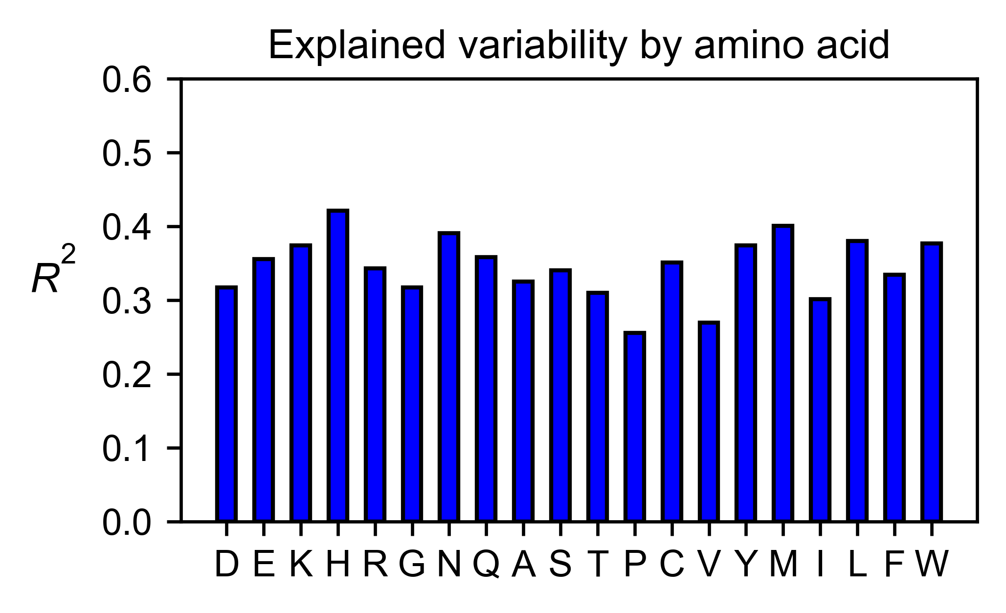
# Explained variability by amino acid
ube2i_obj.individual_correlation(
yscale=[0, 0.6],
title='Explained variability by amino acid',
)
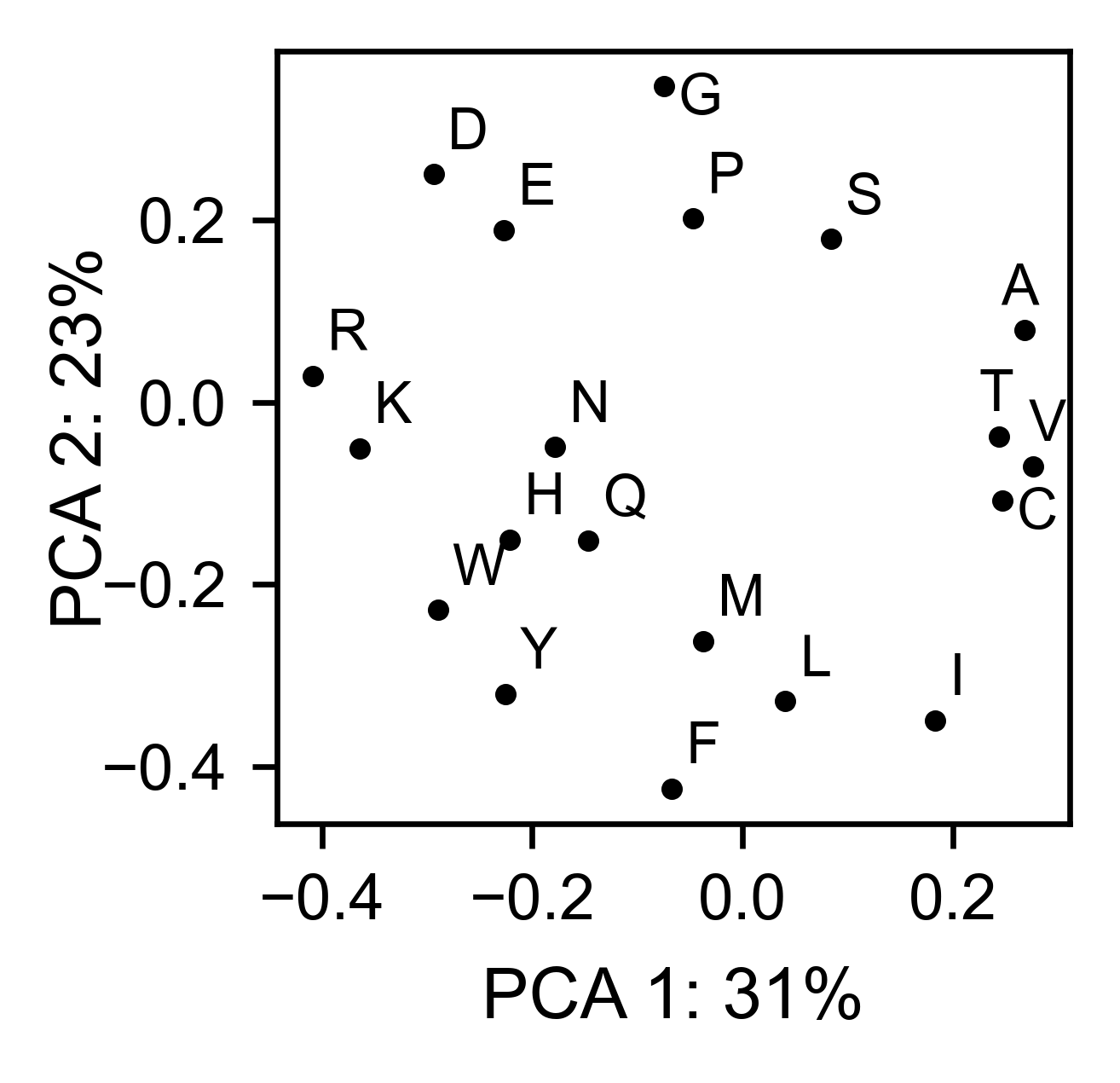
# PCA by amino acid substitution
ube2i_obj.pca(
title='',
dimensions=[0, 1],
figsize=(2, 2),
adjustlabels=True,
)
# PCA by secondary structure motif
ube2i_obj.pca(
title='',
mode='secondary',
dimensions=[0, 1],
figsize=(2, 2),
adjustlabels=True,
)
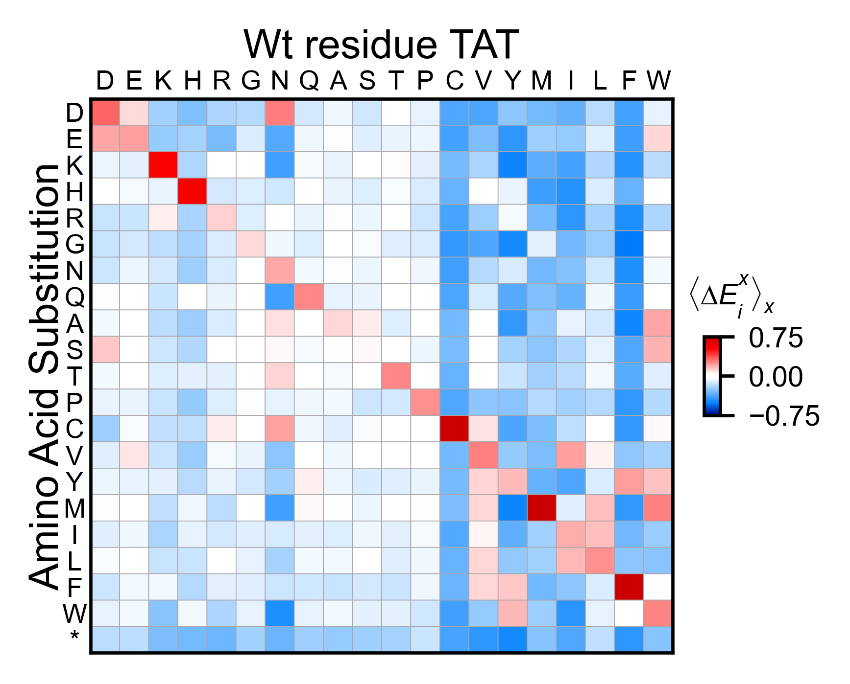
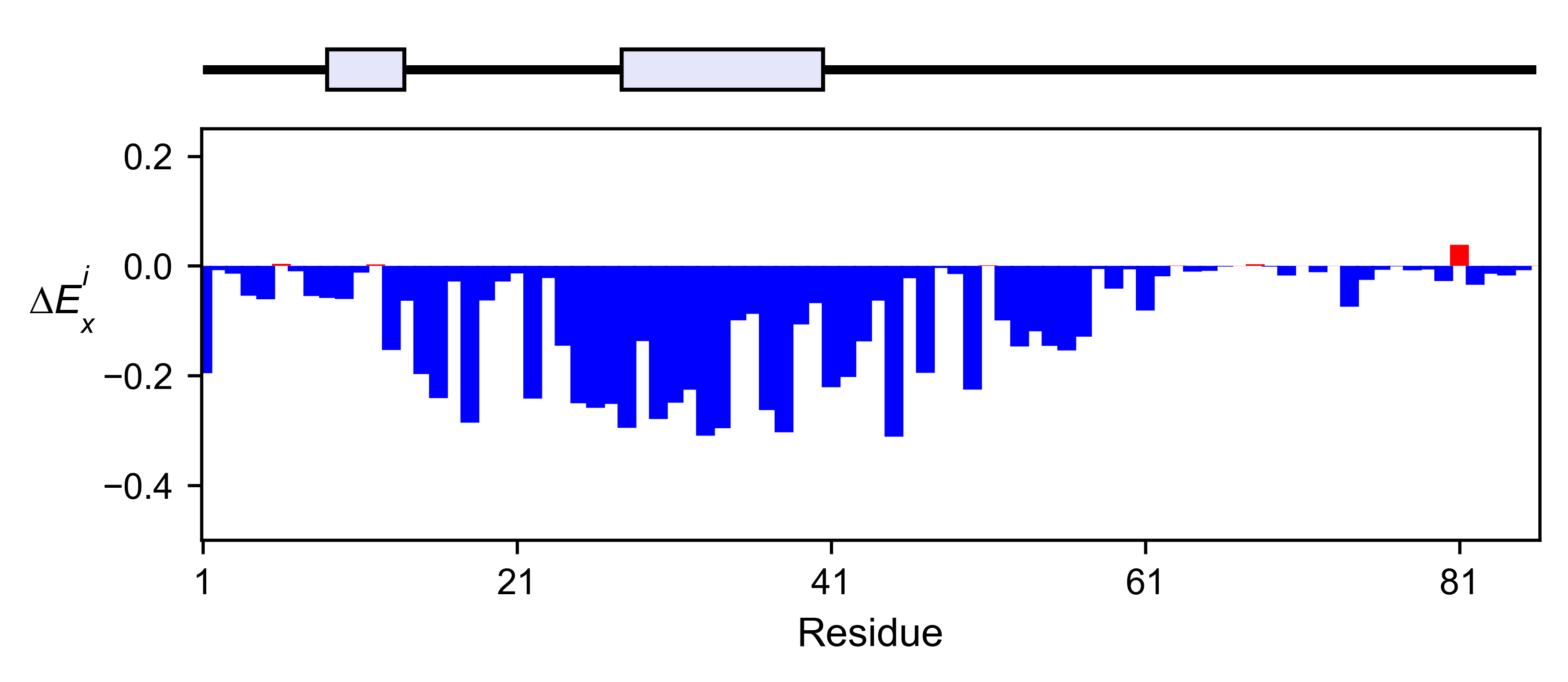
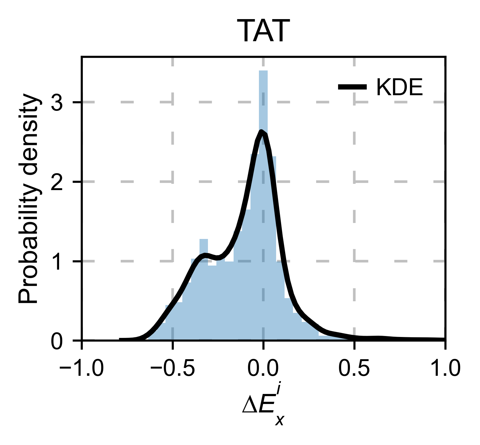
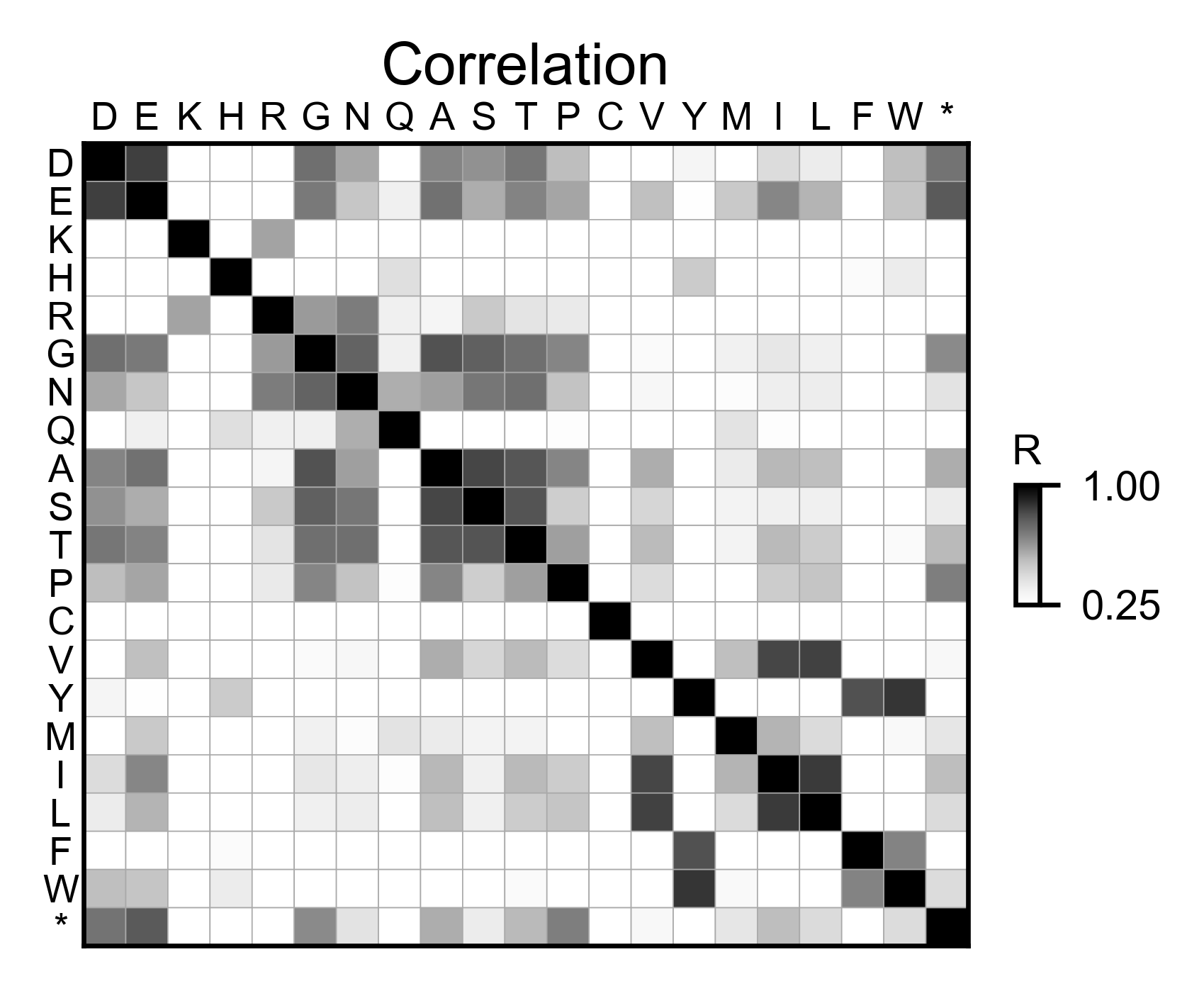
TAT
Create object
#https://doi.org/10.1016/j.cell.2016.11.031
# Order of amino acid substitutions in the hras_enrichment dataset
aminoacids = list(DEMO_DATASETS['df_tat'].index)
# First residue of the hras_enrichment dataset. Because 1-Met was not mutated, the dataset starts at residue 2
start_position = DEMO_DATASETS['df_tat'].columns[0]
# Full sequence
sequence_tat = 'MEPVDPRLEPWKHPGSQPKTACTNCYCKKCCFHCQVCFITKALGISYGRKKRRQRRRAHQ' + 'NSQTHQASLSKQPTSQPRGDPTGPKE'
# Define secondary structure
secondary_tat = [['L1'] * (8), ['α1'] * (13 - 8), ['L2'] * (28 - 14), ['α2'] * (41 - 28),
['L3'] * (90 - 41)]
tat_obj: Screen = Screen(
DEMO_DATASETS['df_tat'], sequence_tat, aminoacids, start_position, 0, secondary_tat
)
2D Plots
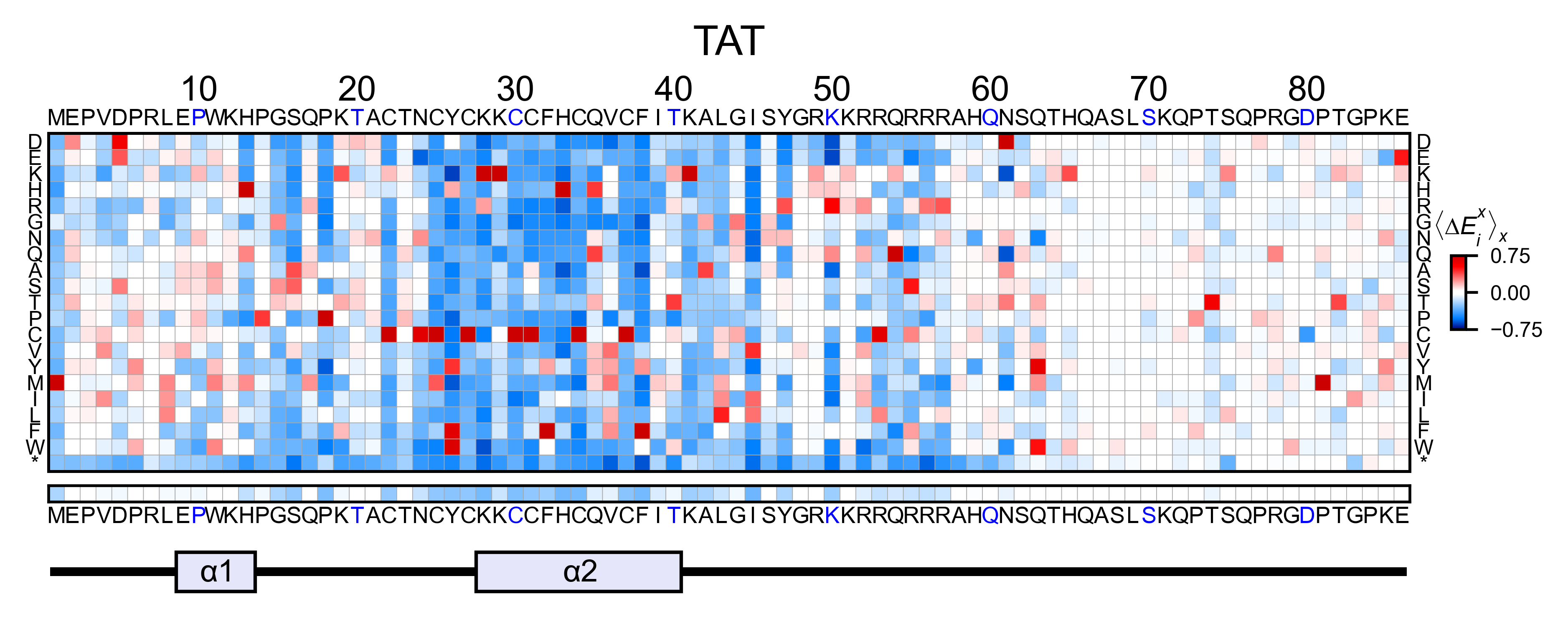
# Create full heatmap
tat_obj.heatmap(
colorbar_scale=(-0.75, 0.75),
neworder_aminoacids=neworder_aminoacids,
title='TAT',
show_cartoon=True,
)
# Miniheatmap
tat_obj.miniheatmap(
title='Wt residue TAT',
colorbar_scale=(-0.75, 0.75),
neworder_aminoacids=neworder_aminoacids,
)
# Positional mean
tat_obj.enrichment_bar(
figsize=[6, 2.5],
mode='mean',
show_cartoon=True,
yscale=[-0.5, 0.25],
title='',
)
# Kernel
tat_obj.kernel(histogram=True, title='TAT', xscale=[-1, 1], output_file=None)
# Correlation between amino acids
tat_obj.correlation(
colorbar_scale=[0.25, 1],
title='Correlation',
neworder_aminoacids=neworder_aminoacids,
)
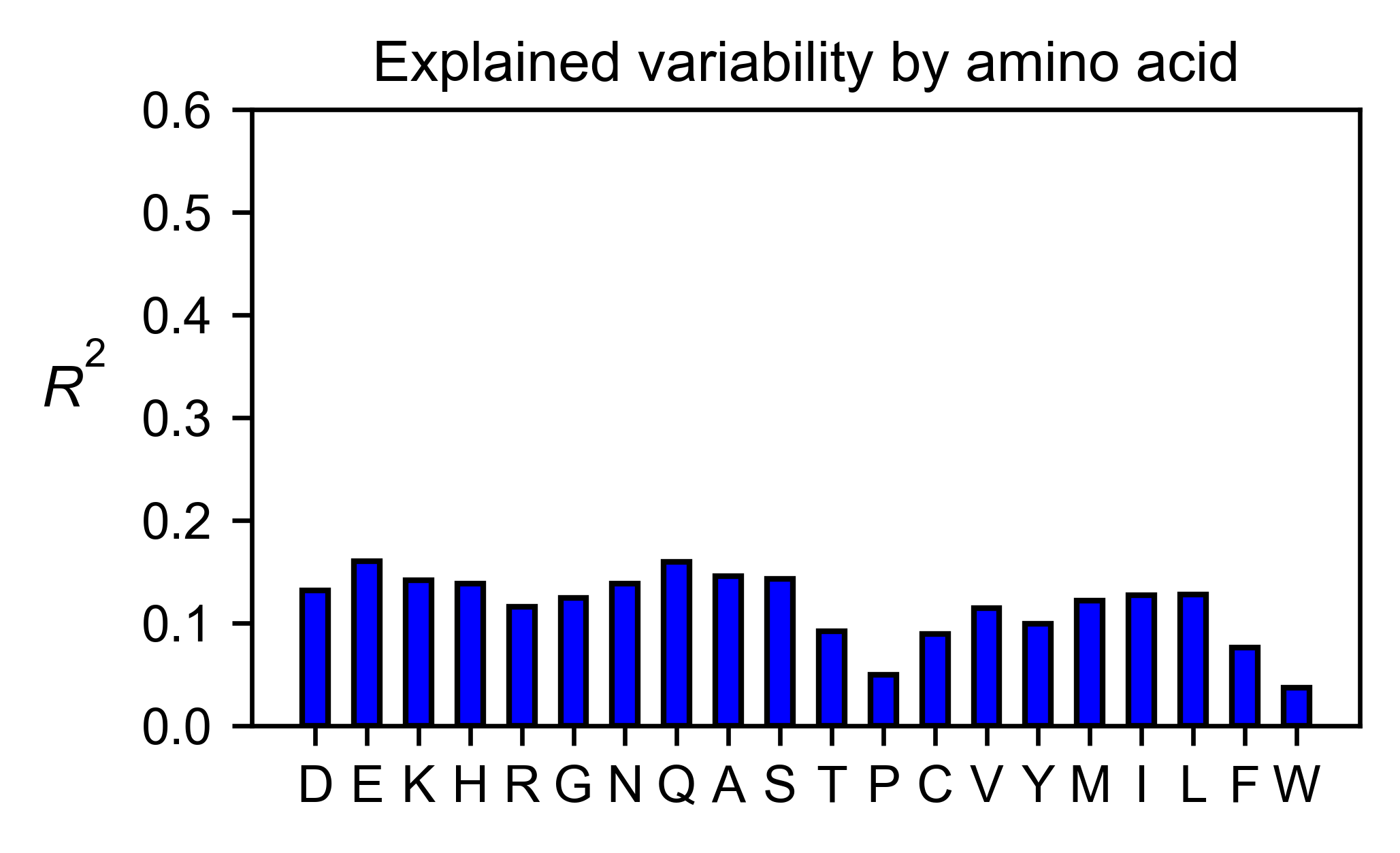
# Explained variability by amino acid
tat_obj.individual_correlation(
yscale=[0, 0.6],
title='Explained variability by amino acid',
)
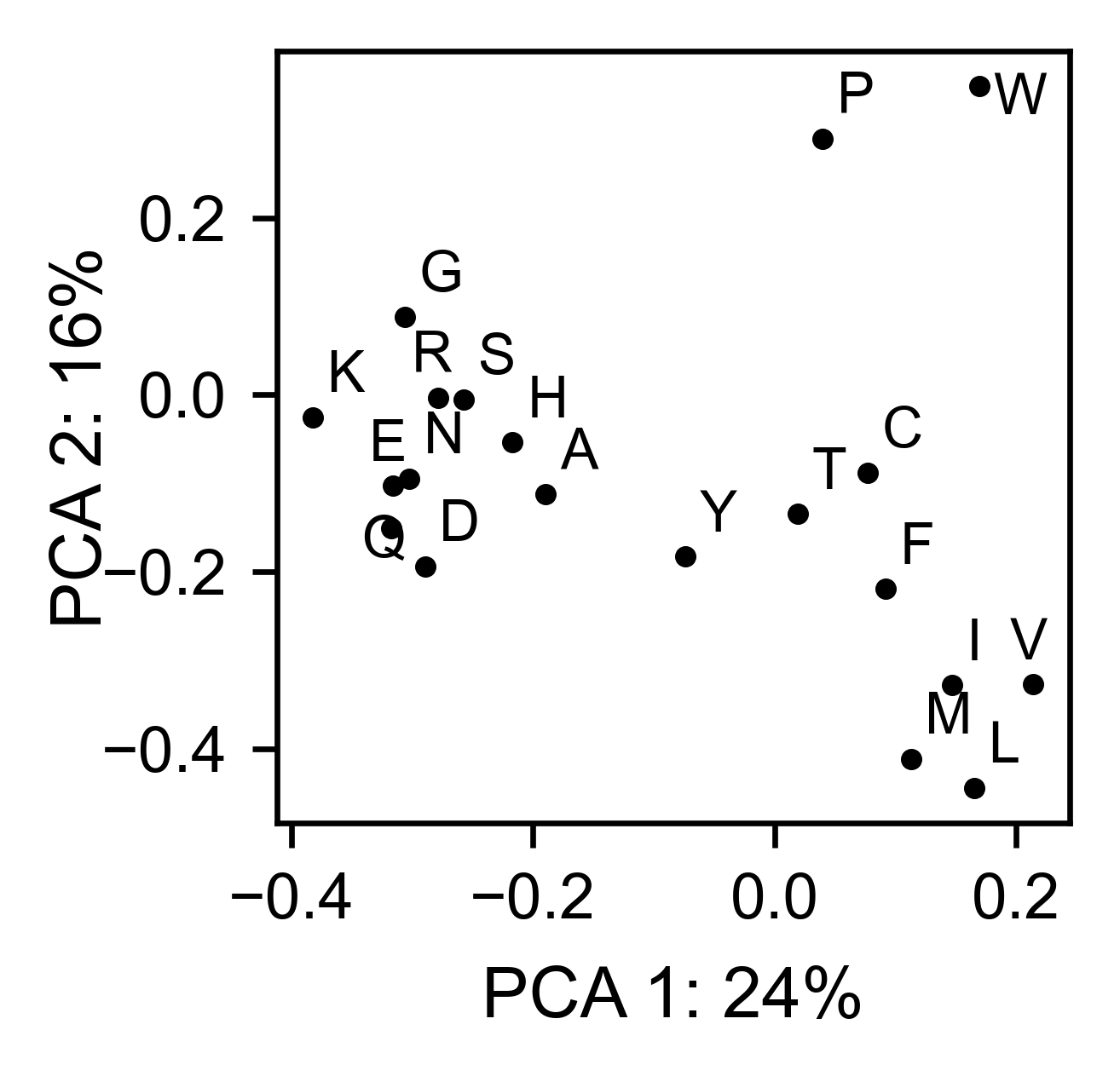
# PCA by amino acid substitution
tat_obj.pca(
title='',
dimensions=[0, 1],
figsize=(2, 2),
adjustlabels=True,
)
REV
Create object
#https://doi.org/10.1016/j.cell.2016.11.031
#https://www.uniprot.org/uniprot/P69718
# Order of amino acid substitutions in the hras_enrichment dataset
aminoacids = list(DEMO_DATASETS['df_rev'].index)
# First residue of the hras_enrichment dataset. Because 1-Met was not mureved, the dataset starts at residue 2
start_position = DEMO_DATASETS['df_rev'].columns[0]
# Full sequence
sequence_rev = 'MAGRSGDSDEDLLKAVRLIKFLYQSNPPPNPEGTRQARRNRRRRWRERQRQIHSISERIL' + 'STYLGRSAEPVPLQLPPLERLTLDCNEDCGTSGTQGVGSPQILVESPTILESGAKE'
# Define secondary structure
secondary_rev = [['L1'] * (8), ['α1'] * (25 - 8), ['L2'] * (33 - 25), ['α2'] * (68 - 33),
['L3'] * (116 - 41)]
rev_obj: Screen = Screen(
DEMO_DATASETS['df_rev'], sequence_rev, aminoacids, start_position, 0, secondary_rev
)
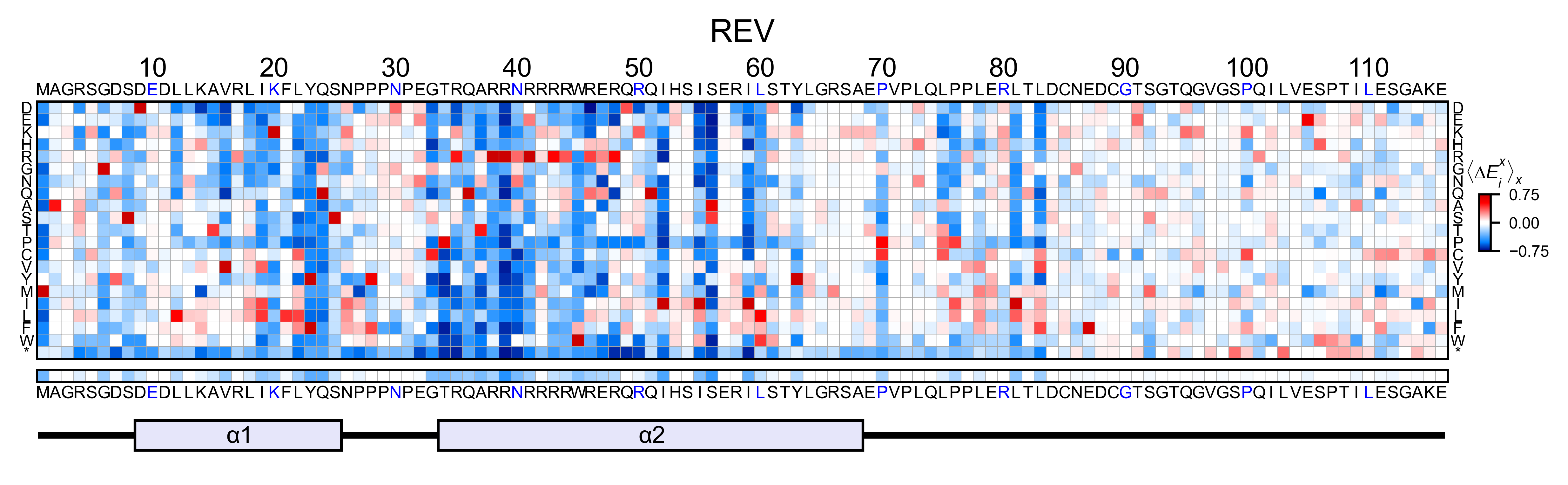
2D Plots
# Create full heatmap
rev_obj.heatmap(
colorbar_scale=(-0.75, 0.75),
neworder_aminoacids=neworder_aminoacids+["*"],
title='REV',
show_cartoon=True,
)
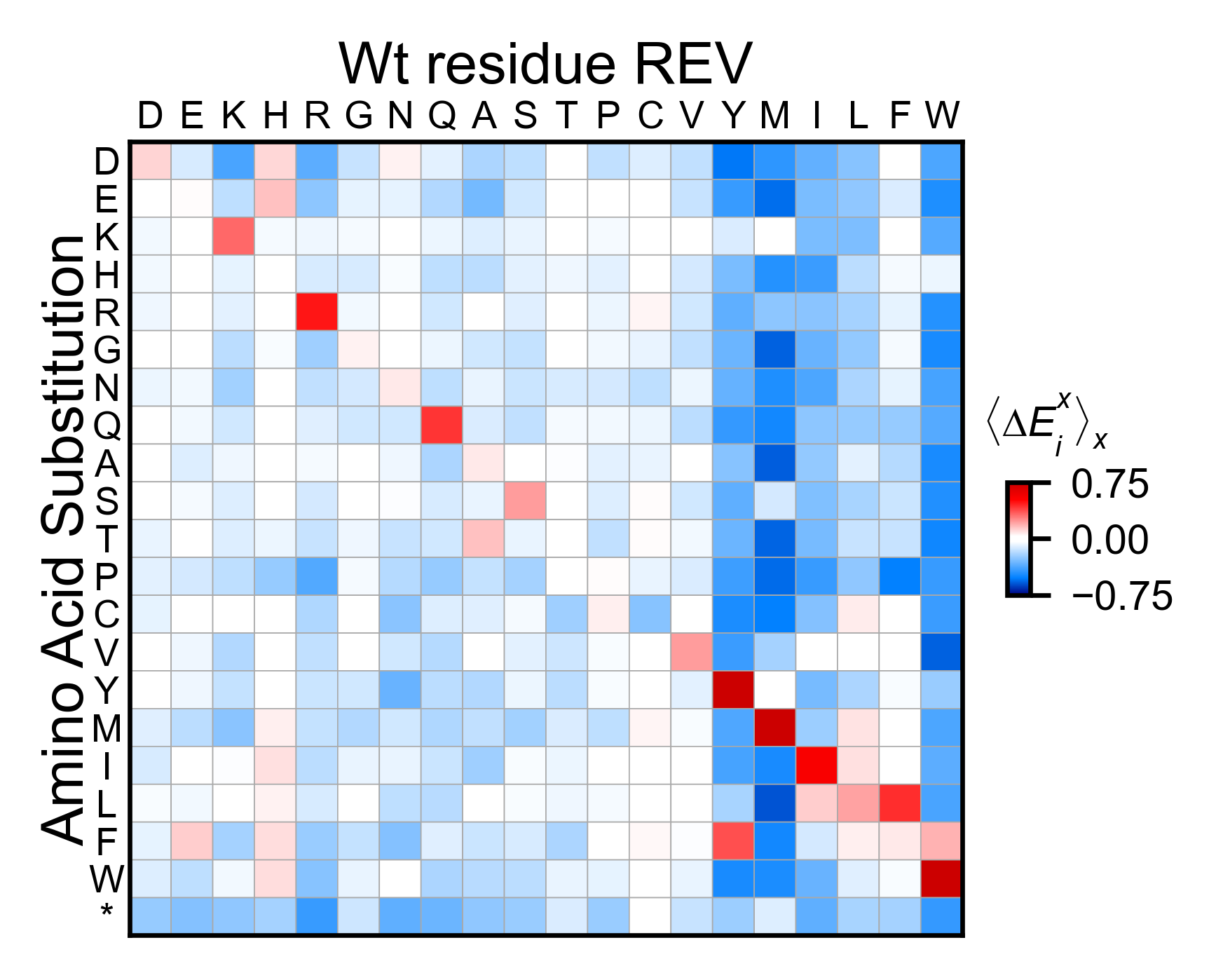
# Miniheatmap
rev_obj.miniheatmap(
title='Wt residue REV',
colorbar_scale=(-0.75, 0.75),
neworder_aminoacids=neworder_aminoacids+["*"],
)
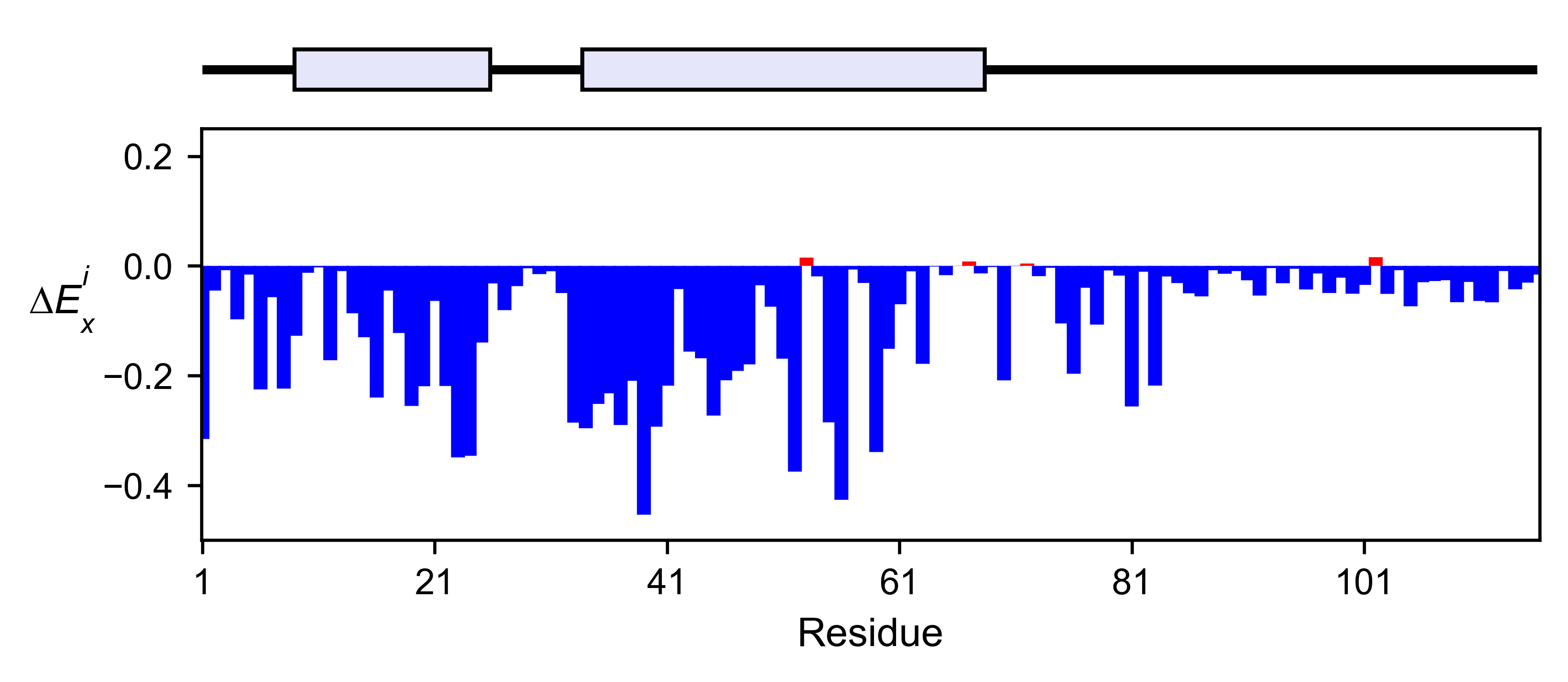
# Positional mean
rev_obj.enrichment_bar(
figsize=[6, 2.5],
mode='mean',
show_cartoon=True,
yscale=[-0.5, 0.25],
title='',
)
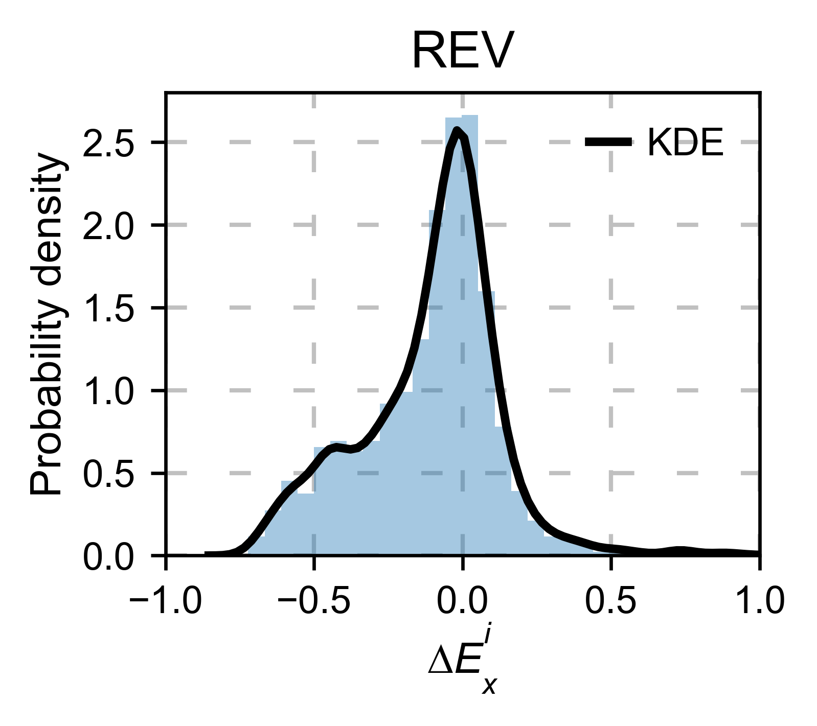
# Kernel
rev_obj.kernel(histogram=True, title='REV', xscale=[-1, 1], output_file=None)
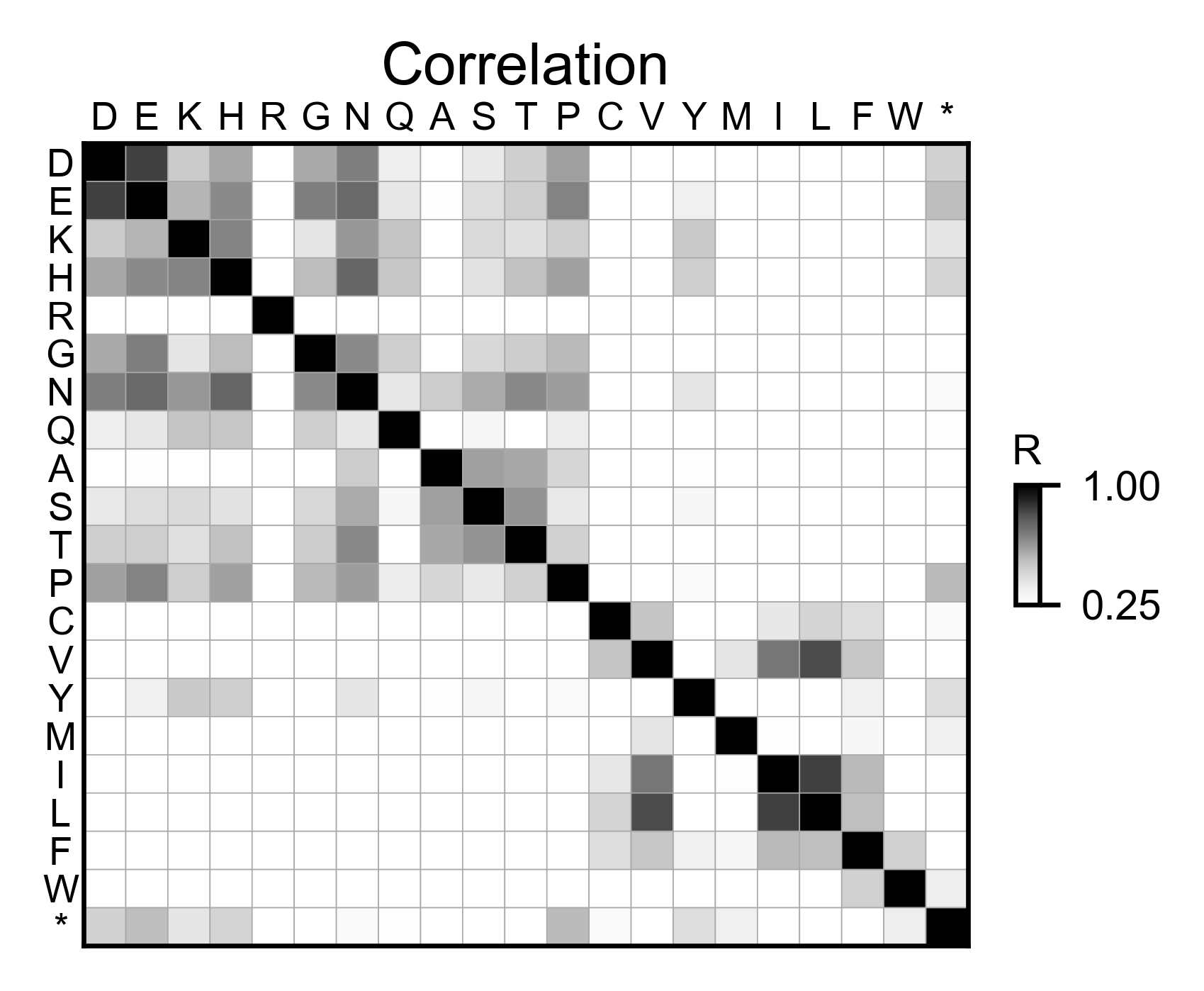
# Correlation between amino acids
rev_obj.correlation(
colorbar_scale=[0.25, 1],
title='Correlation',
neworder_aminoacids=neworder_aminoacids,
)
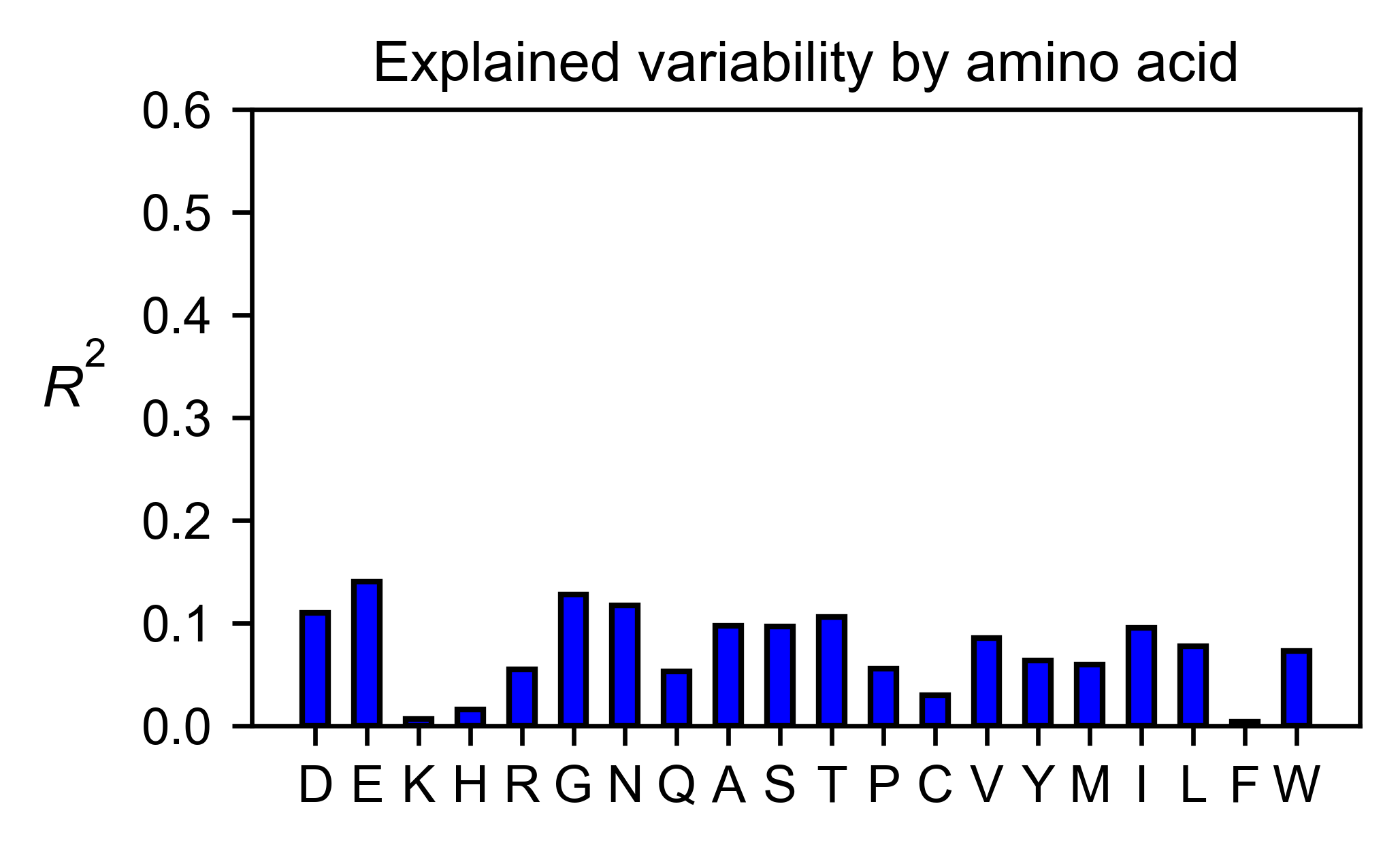
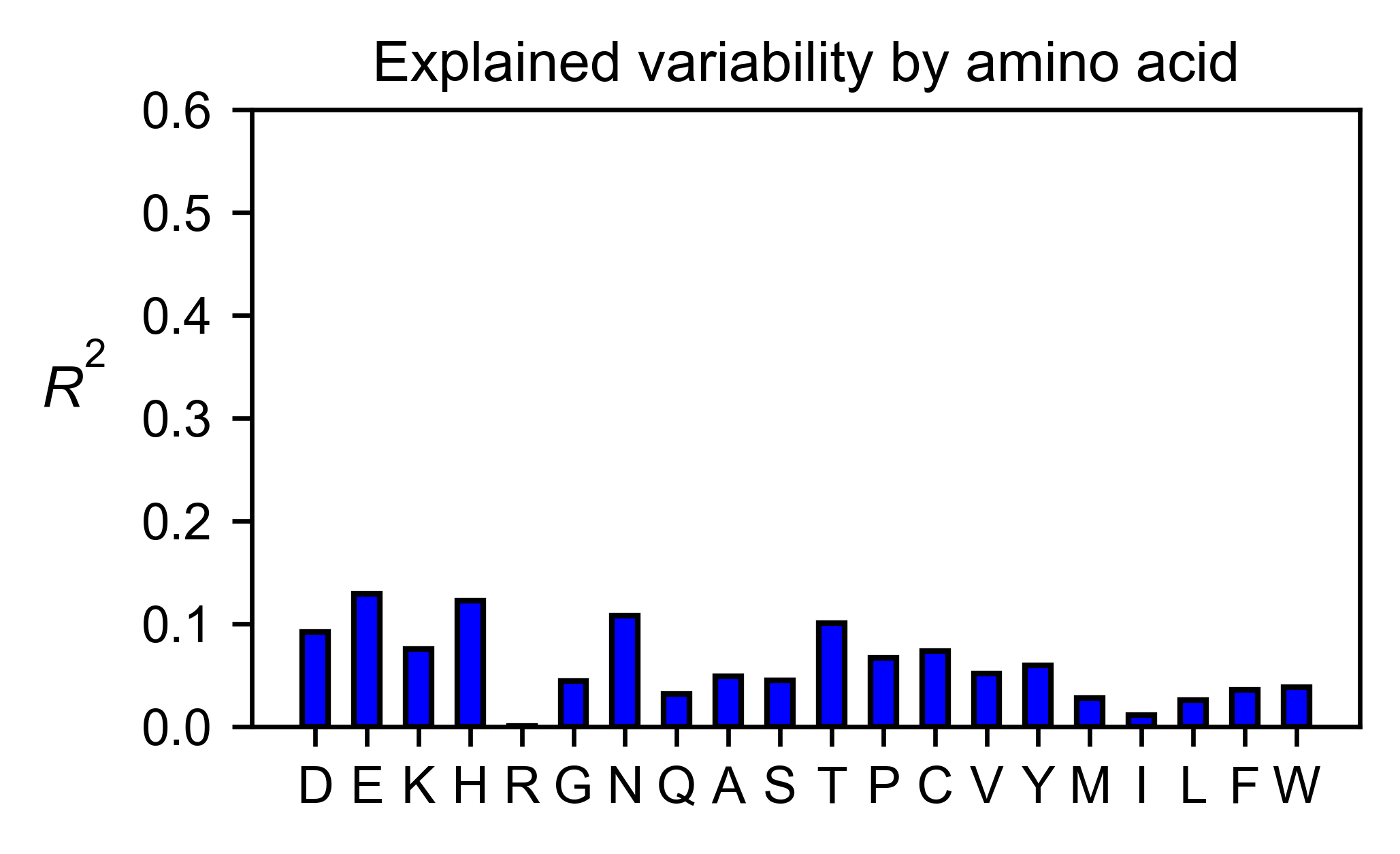
# Explained variability by amino acid
rev_obj.individual_correlation(
yscale=[0, 0.6],
title='Explained variability by amino acid',
)
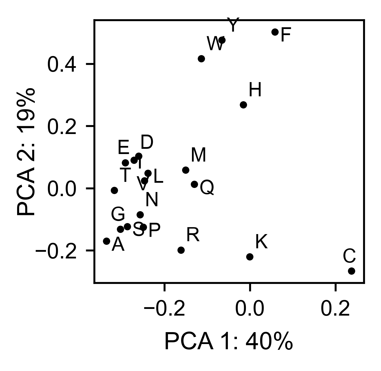
# PCA by amino acid substitution
rev_obj.pca(
title='',
dimensions=[0, 1],
figsize=(2, 2),
adjustlabels=True,
)
α-synuclein
Load data
#https://www.uniprot.org/uniprot/P37840#sequences
#https://doi.org/10.1038/s41589-020-0480-6
# Order of amino acid substitutions in the hras_enrichment dataset
aminoacids = list(DEMO_DATASETS['df_asynuclein'].index)
# First residue of the hras_enrichment dataset. Because 1-Met was not mureved, the dataset starts at residue 2
start_position = DEMO_DATASETS['df_asynuclein'].columns[0]
# Full sequence
sequence_asynuclein = 'MDVFMKGLSKAKEGVVAAAEKTKQGVAEAAGKTKEGVLYVGSKTKEGVVHGVATVAEKTK' + 'EQVTNVGGAVVTGVTAVAQKTVEGAGSIAAATGFVKKDQLGKNEEGAPQEGILEDMPVDP' + 'DNEAYEMPSEEGYQDYEPEA'
# Define secondary structure
secondary_asynuclein = [['L1'] * (1), ['α1'] * (37 - 1), ['L2'] * (44 - 37),
['α2'] * (92 - 44), ['L3'] * (140 - 92)]
asynuclein_obj: Screen = Screen(
DEMO_DATASETS['df_asynuclein'], sequence_asynuclein, aminoacids, start_position, 0,
secondary_asynuclein
)
2D Plots
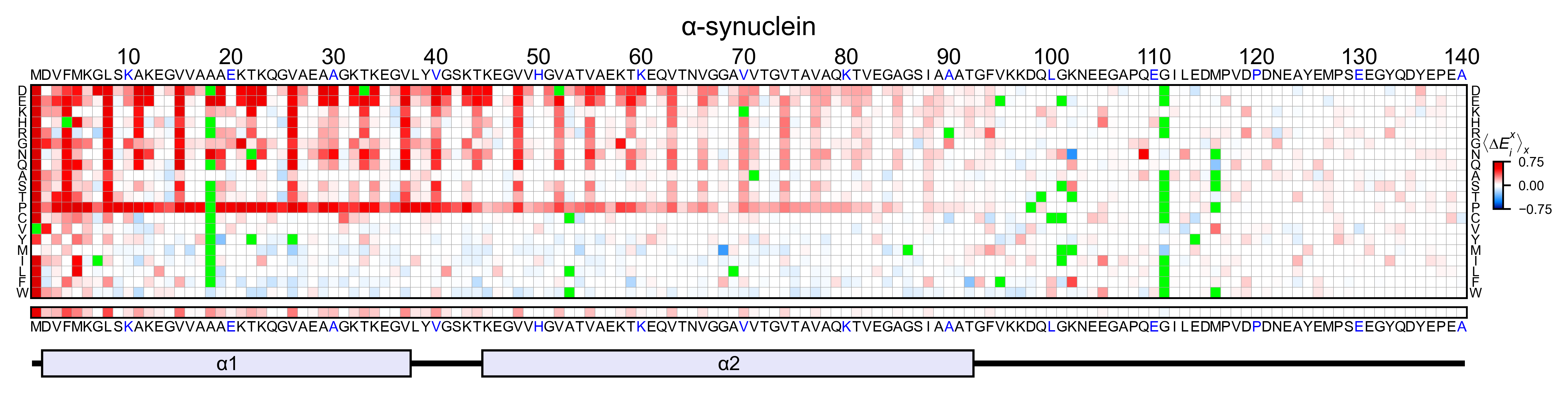
# Create full heatmap
asynuclein_obj.heatmap(
colorbar_scale=(-0.75, 0.75),
neworder_aminoacids=neworder_aminoacids,
title='α-synuclein',
show_cartoon=True,
)
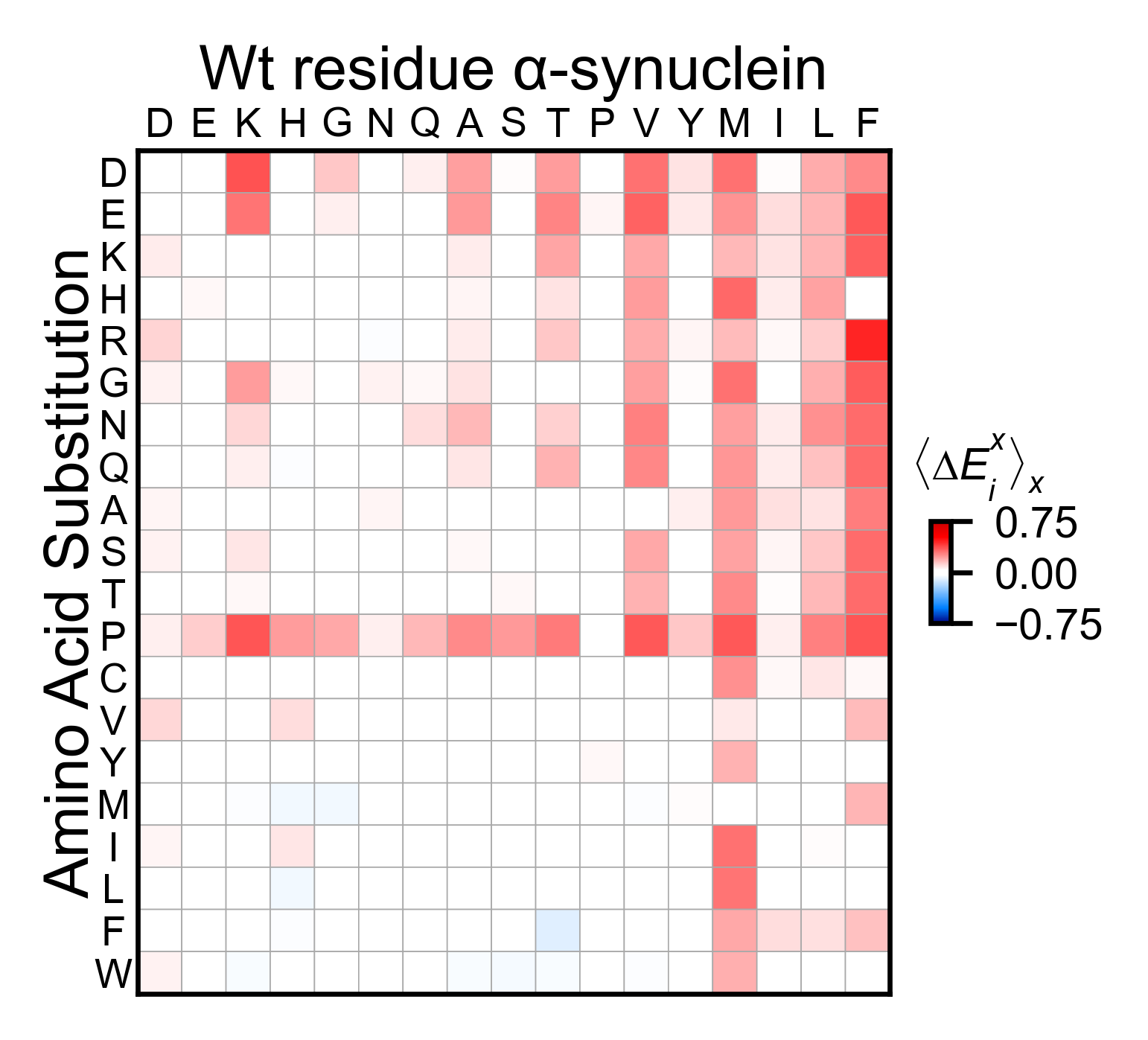
# Miniheatmap
asynuclein_obj.miniheatmap(
title='Wt residue α-synuclein',
colorbar_scale=(-0.75, 0.75),
neworder_aminoacids=neworder_aminoacids,
)
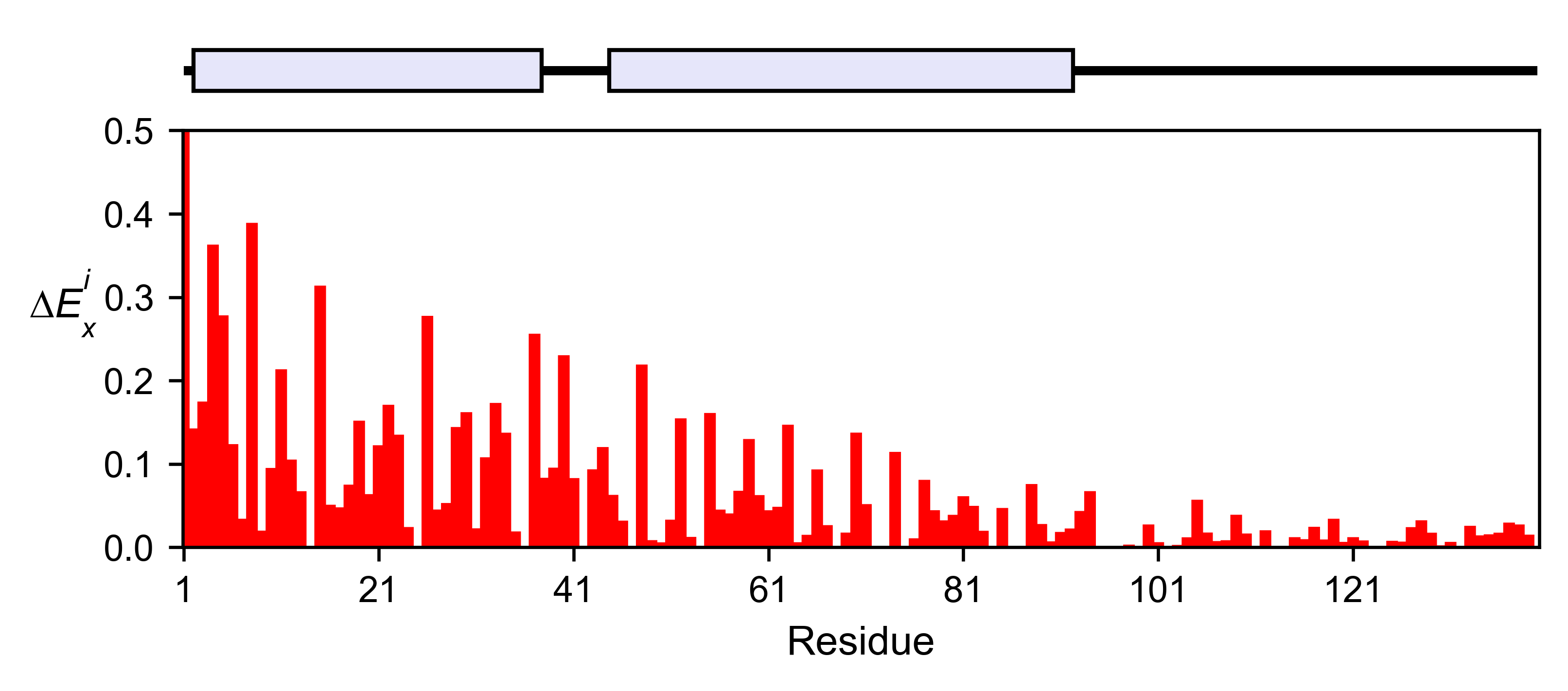
# Positional mean
asynuclein_obj.enrichment_bar(
figsize=[6, 2.5],
mode='mean',
show_cartoon=True,
yscale=[0, 0.5],
title='',
)
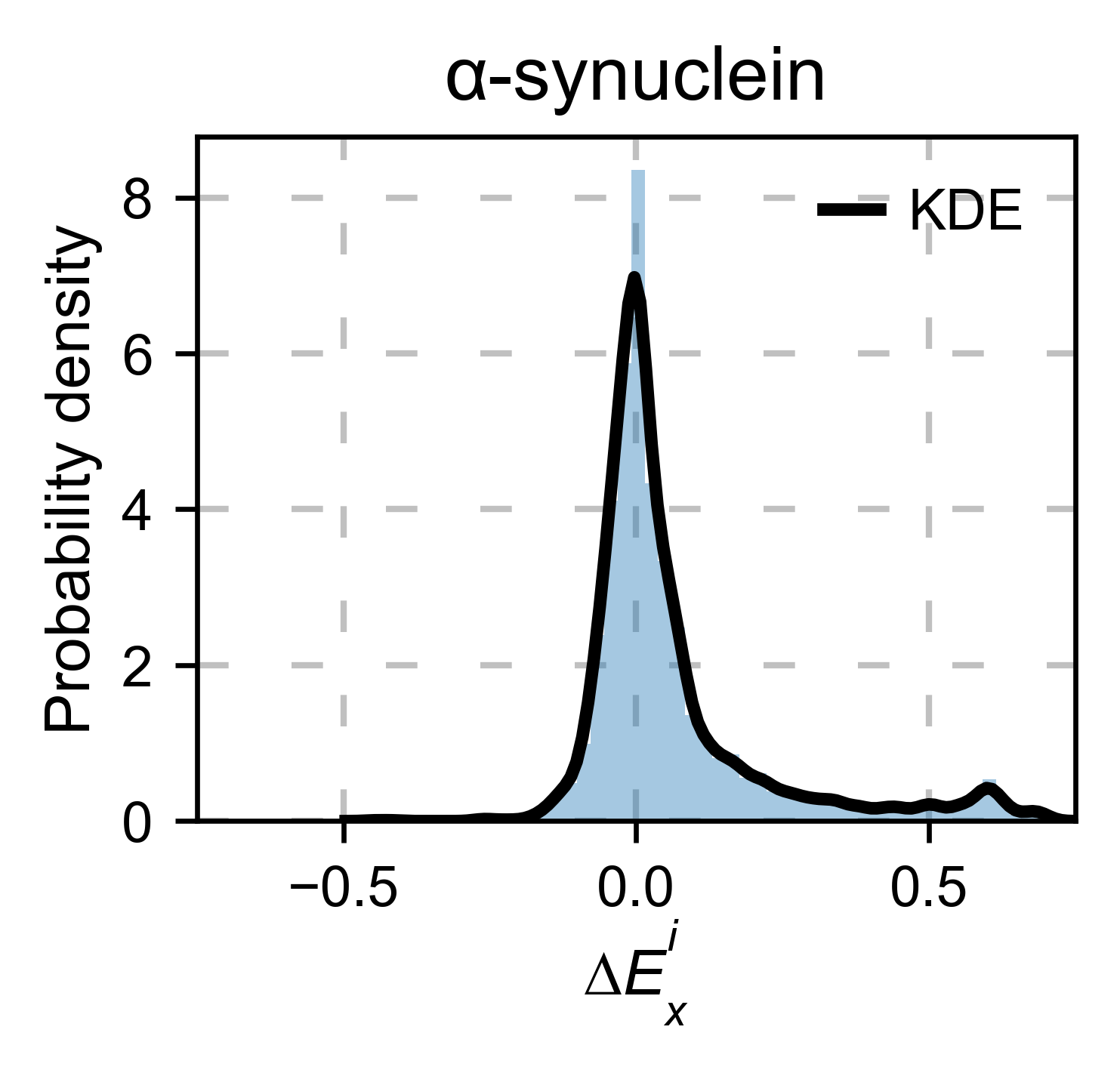
# Kernel
asynuclein_obj.kernel(
histogram=True, title='α-synuclein', xscale=[-0.75, 0.75], output_file=None
)
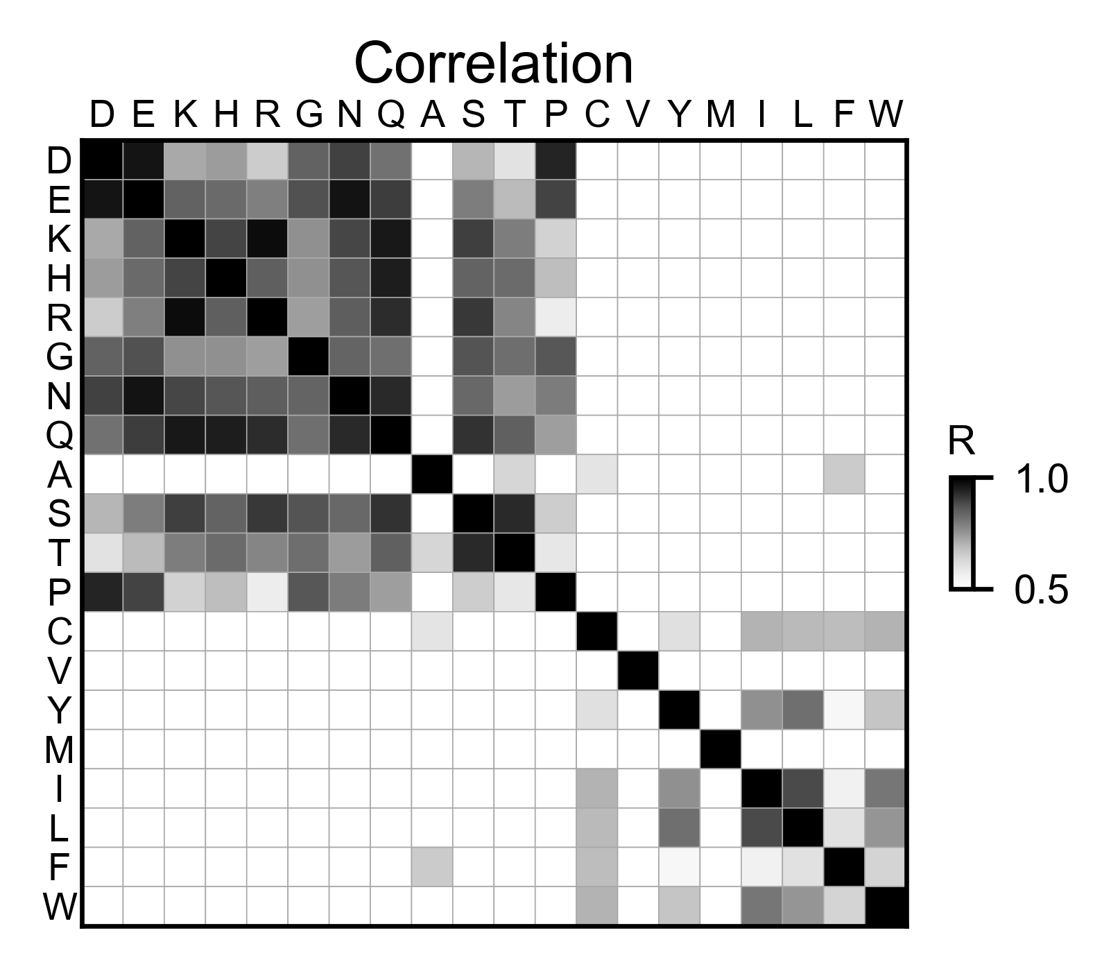
# Correlation between amino acids
asynuclein_obj.correlation(
colorbar_scale=[0.5, 1],
title='Correlation',
neworder_aminoacids=neworder_aminoacids,
)
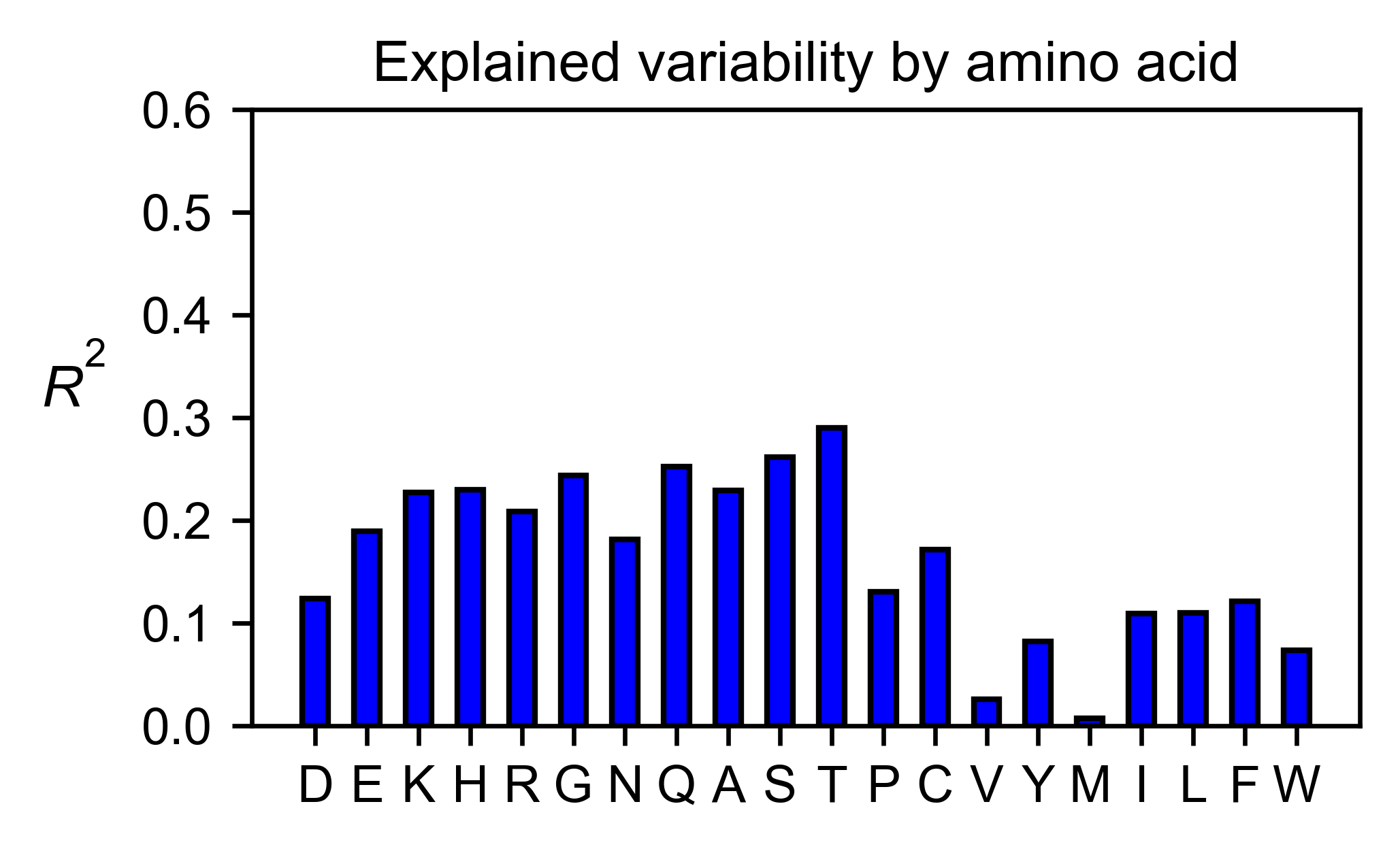
# Explained variability by amino acid
asynuclein_obj.individual_correlation(
yscale=[0, 0.6],
title='Explained variability by amino acid',
)
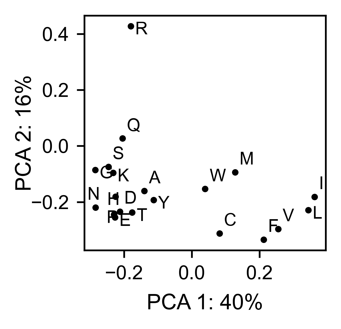
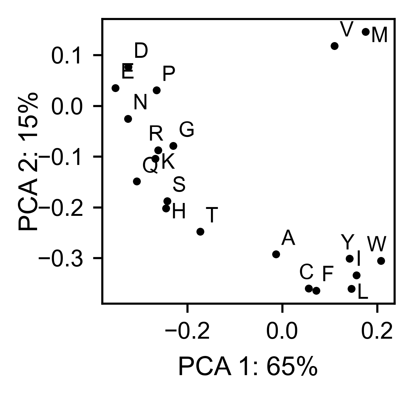
# PCA by amino acid substitution
asynuclein_obj.pca(
title='',
dimensions=[0, 1],
figsize=(2, 2),
adjustlabels=True,
)
APH(3) II
Create object
#https://doi.org/10.1093/nar/gku511
aminoacids = list(DEMO_DATASETS['df_aph'].index)
# First residue of the hras_enrichment dataset. Because 1-Met was not mureved, the dataset starts at residue 2
start_position = DEMO_DATASETS['df_aph'].columns[0]
# Full sequence
sequence_aph = 'MIEQDGLHAGSPAAWVERLFGYDWAQQTIGCSDAAVFRLSAQGRPVLFVKTDLSGALNELQ' + 'DEAARLSWLATTGVPCAAVLDVVTEAGRDWLLLGEVPGQDLLSSHLAPAEKVSIMADAMRR' + 'LHTLDPATCPFDHQAKHRIERARTRMEAGLVDQDDLDEEHQGLAPAELFARLKARMPDGED' + 'LVVTHGDACLPNIMVENGRFSGFIDCGRLGVADRYQDIALATRDIAEELGGEWADRFLVLY' + 'GIAAPDSQRIAFYRLLDEFF'
# Define secondary structure
secondary_aph = [['L1'] * (11), ['α1'] * (16 - 11), ['L2'] * (22 - 16), ['β1'] * (26 - 22),
['L3'] * (34 - 26), ['β2'] * (40 - 34), ['L4'] * (46 - 40), ['β3'] *
(52 - 46), ['L5'] * (58 - 52), ['α2'] * (72 - 58), ['L6'] * (79 - 72),
['β4'] * (85 - 79), ['L7'] * (89 - 85), ['β5'] * (95 - 89),
['L8'] * (99 - 95), ['β6'] * (101 - 99), ['L9'] * (107 - 101),
['α3'] * (131 - 107), ['L10'] * (135 - 131), ['α4'] * (150 - 135),
['L11'] * (158 - 150), ['α5'] * (163 - 158), ['L12'] * (165 - 163),
['α6'] * (177 - 165), ['L13'] * (183 - 177), ['β7'] * (187 - 183),
['L14'] * (191 - 187), ['α7'] * (194 - 191), ['L15'] * (1),
['β8'] * (199 - 195), ['L16'] * (201 - 199), ['β9'] * (206 - 201),
['L17'] * (212 - 206), ['β10'] * (216 - 212), ['α8'] * (245 - 216),
['L18'] * (4), ['α9'] * (264 - 249)]
aph_obj: Screen = Screen(
np.log10(DEMO_DATASETS['df_aph']), sequence_aph, aminoacids, start_position, 0,
secondary_aph
)
2D Plots
colormap = copy.copy((plt.cm.get_cmap('Blues_r')))
# Create full heatmap
aph_obj.heatmap(
colorbar_scale=(-0.75, 0.25),
neworder_aminoacids=neworder_aminoacids,
title='APH',
show_cartoon=True,
colormap=colormap,
)
# Miniheatmap
aph_obj.miniheatmap(
title='Wt residue APH',
neworder_aminoacids=neworder_aminoacids,
colormap=colormap,
colorbar_scale=(-0.75, 0.25),
)
# Positional mean
aph_obj.enrichment_bar(
figsize=[10, 2.5],
mode='mean',
show_cartoon=True,
yscale=[-1.5, 0.5],
title='',
)
# Kernel
aph_obj.kernel(histogram=True, title='APH', xscale=[-2, 2], output_file=None)
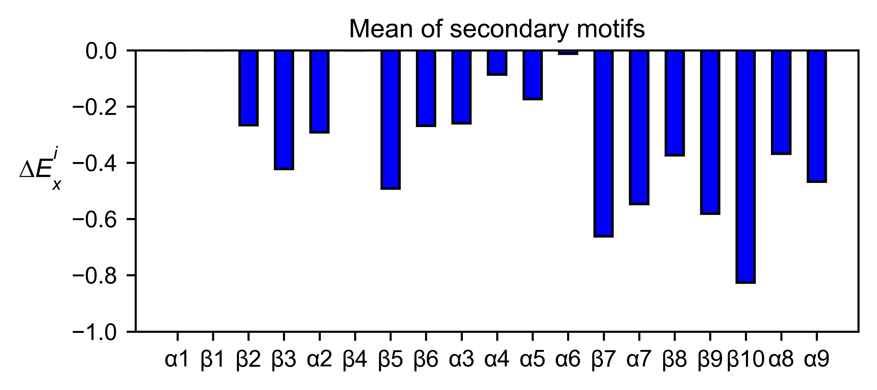
# Graph bar of the mean of each secondary motif
aph_obj.secondary_mean(
yscale=[-1, 0],
figsize=[5, 2],
title='Mean of secondary motifs',
)
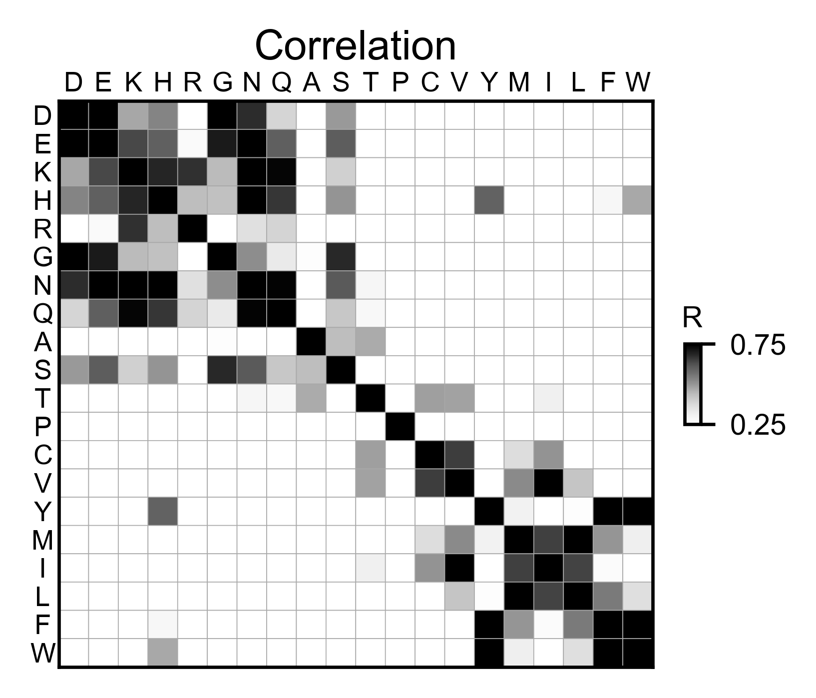
# Correlation between amino acids
aph_obj.correlation(
colorbar_scale=[0.25, 0.75],
title='Correlation',
neworder_aminoacids=neworder_aminoacids,
)
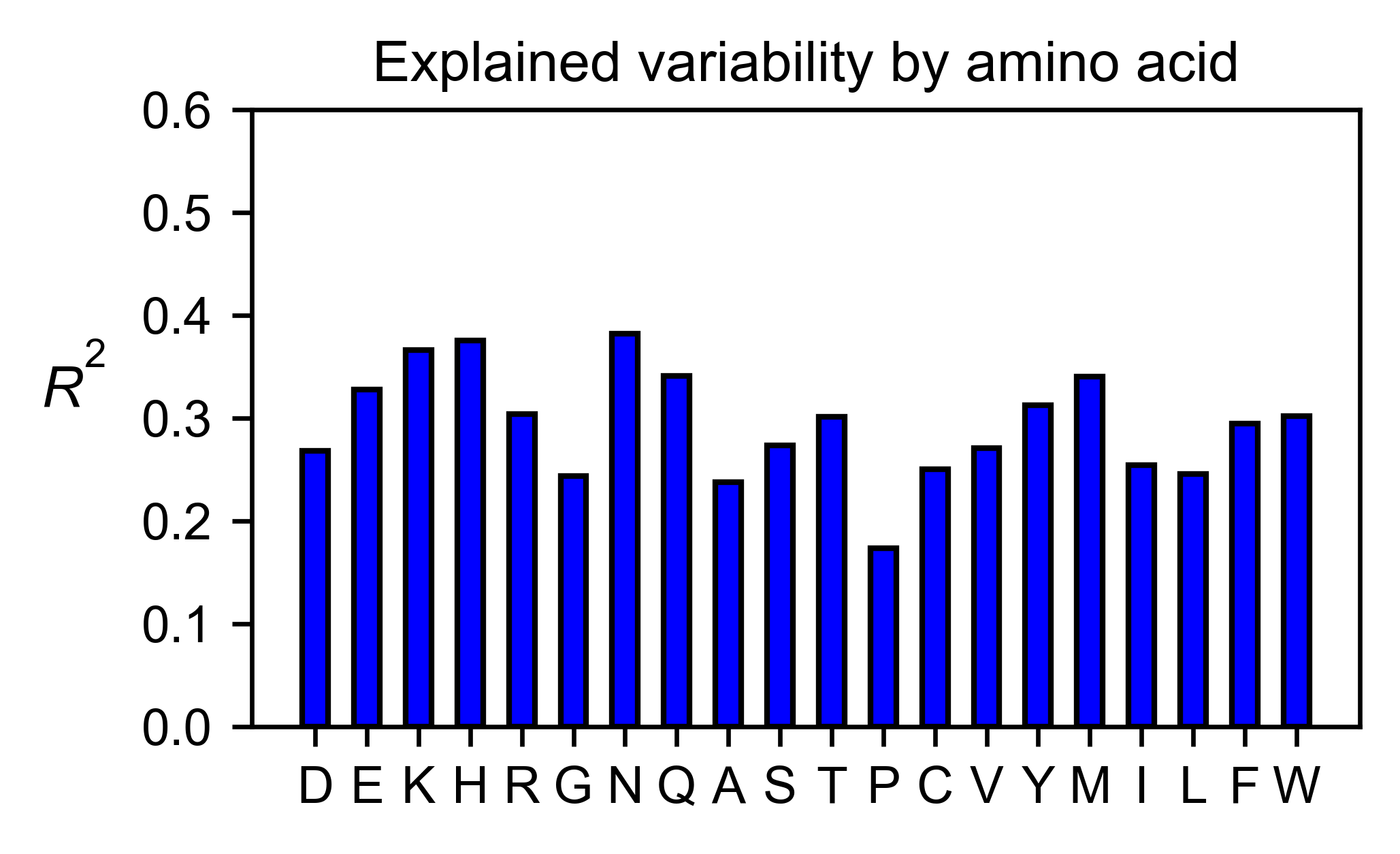
# Explained variability by amino acid
aph_obj.individual_correlation(
yscale=[0, 0.6],
title='Explained variability by amino acid',
)
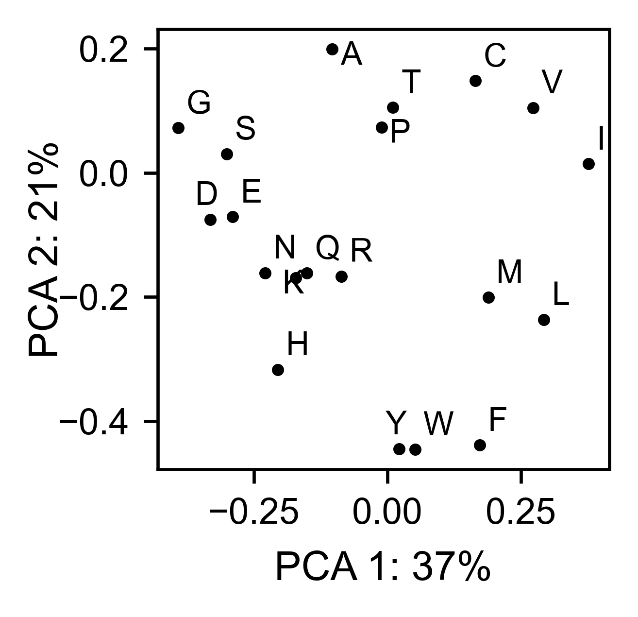
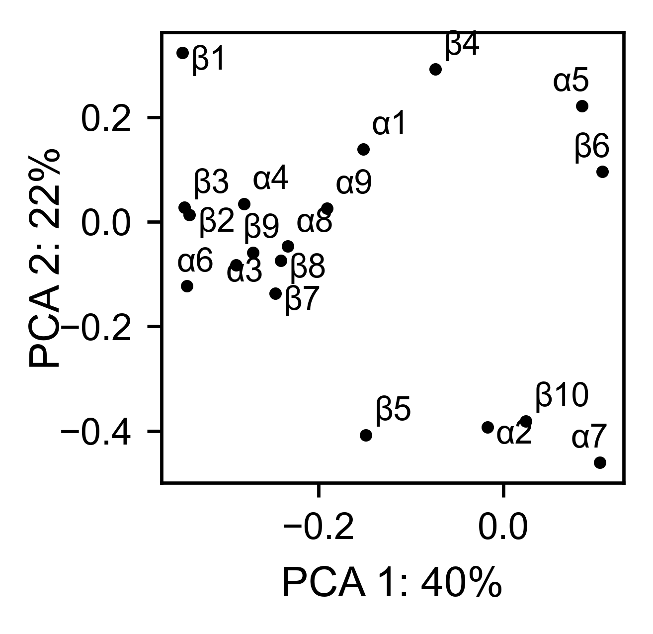
# PCA by amino acid substitution
aph_obj.pca(
title='',
dimensions=[0, 1],
figsize=(2, 2),
adjustlabels=True,
)
# PCA by secondary structure motif
aph_obj.pca(
title='',
mode='secondary',
dimensions=[0, 1],
figsize=(2, 2),
adjustlabels=True,
)
3D plots
colormap = copy.copy((plt.cm.get_cmap('Blues_r')))
# Plot 3-D plot
aph_obj.plotly_scatter_3d(
mode='mean',
pdb_path=PDB_1ND4,
title='Scatter 3D aph',
squared=False,
position_correction=0,
x_label='x',
y_label='y',
z_label='z',
colormap = colormap,
colorbar_scale = (-.75, 0.25),
)
# Plot 3-D of distance to center of protein, SASA and B-factor
aph_obj.plotly_scatter_3d_pdbprop(
plot=['Distance', 'SASA', 'log B-factor'],
position_correction=0,
pdb_path=PDB_1ND4,
title='Scatter 3D - PDB properties',
colorbar_scale = (-.75, 0.25),
colormap = colormap,
)
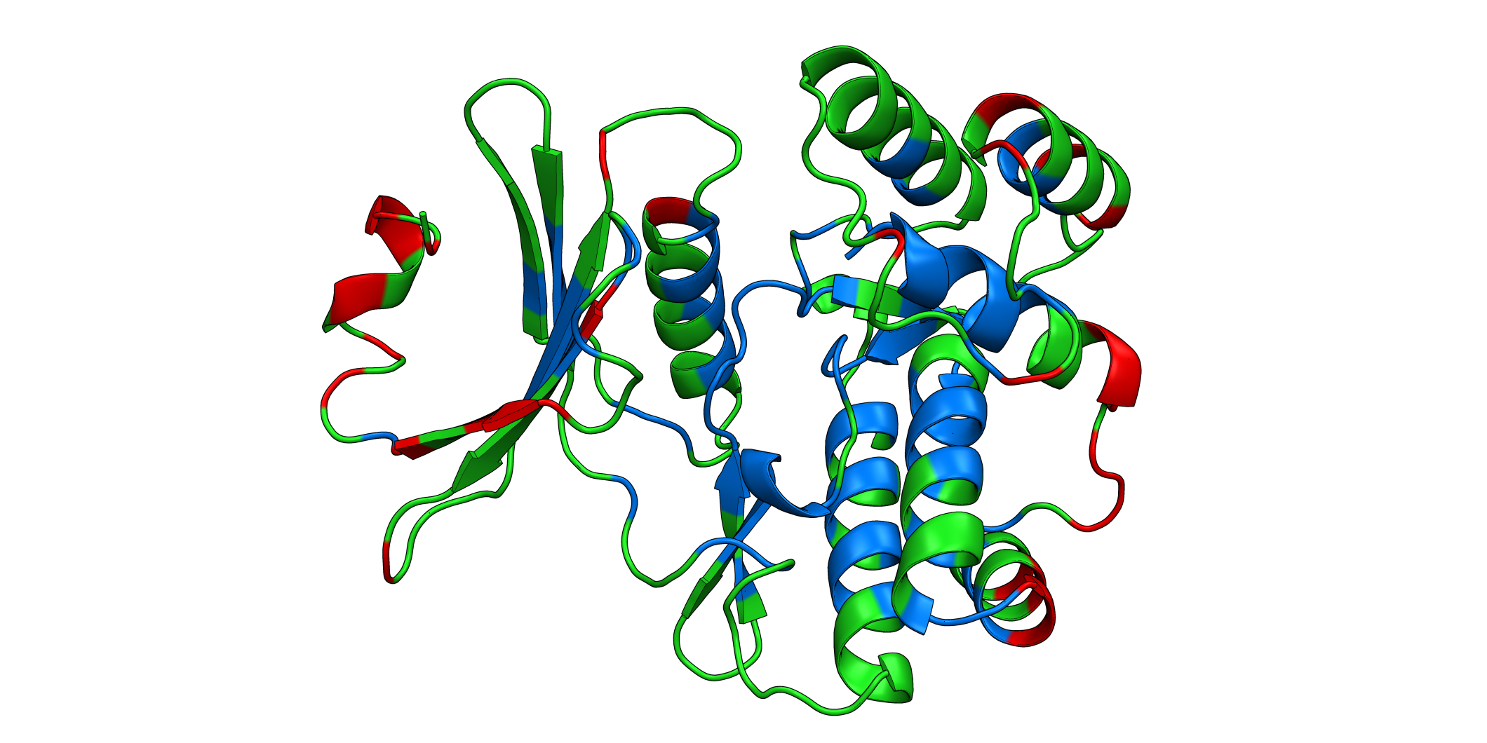
# Start pymol and color residues. Cut offs are set with gof and lof parameters.
aph_obj.pymol(
pdb=PDB_1ND4,
mode='mean',
gof=0.25,
lof=-0.5,
position_correction=0
)
b11l5f
Create object
#https://doi.org/10.5281/zenodo.1216229
# Order of amino acid substitutions in the hras_enrichment dataset
aminoacids = list(DEMO_DATASETS['df_b11l5f'].index)
neworder_aminoacids: List[str] = list('DEKHRGNQASTPVYMILFW')
# Sequence
sequence_b11l5f = 'CRAASLLPGTWQVTMTNEDGQTSQGQMHFQPRSPYTLDVKAQGTISDGRPI' + 'SGKGKVTCKTPDTMDVDITYPSLGNMKVQGQVTLDSPTQFKFDVTTSDGSKVTGTLQRQE'
# First residue of the hras_enrichment dataset. Because 1-Met was not mureved, the dataset starts at residue 2
start_position = DEMO_DATASETS['df_b11l5f'].columns[0]
b11l5f_obj: Screen = Screen(DEMO_DATASETS['df_b11l5f'], sequence_b11l5f, aminoacids, start_position, 0)
2D Plots
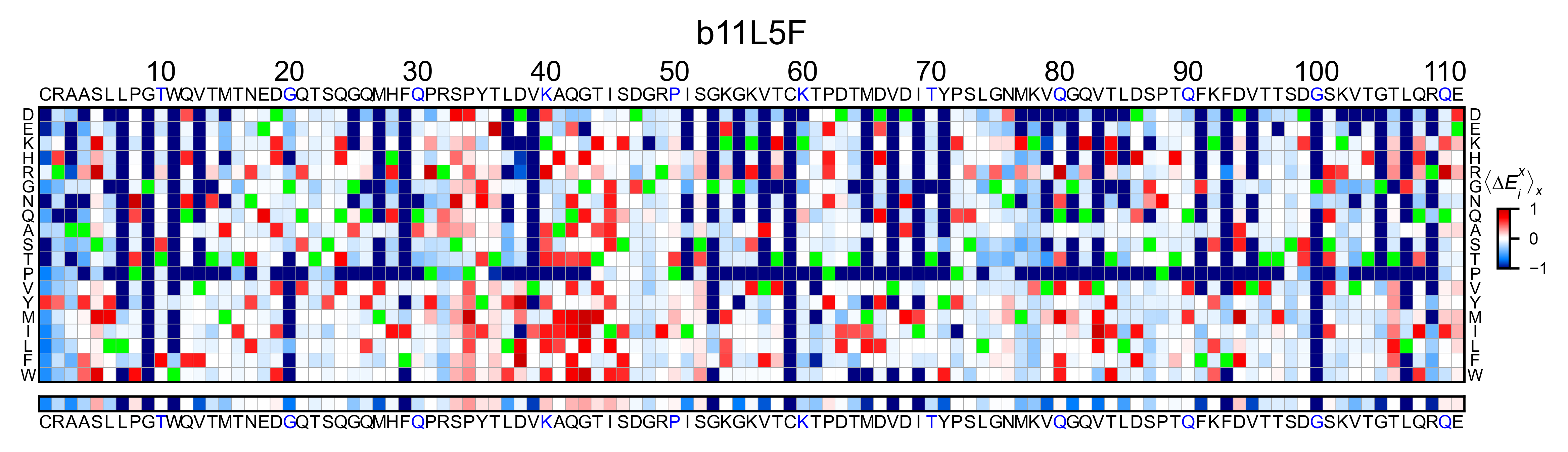
colormap = copy.copy((plt.cm.get_cmap('bwr')))
# Create full heatmap
b11l5f_obj.heatmap(
neworder_aminoacids=neworder_aminoacids, title='b11l5f', output_file=None
)
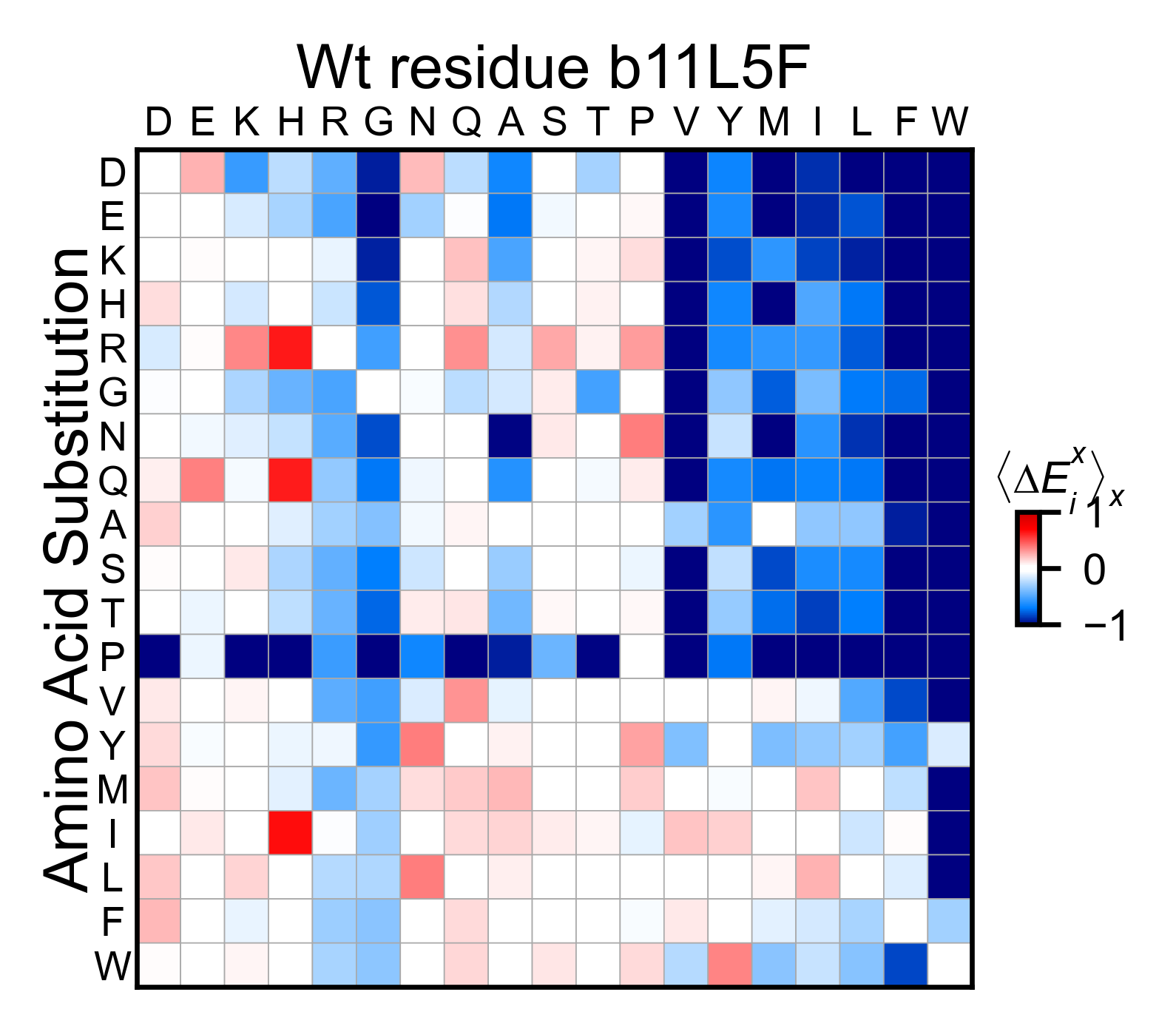
# Miniheatmap
b11l5f_obj.miniheatmap(
title='Wt residue b11l5f',
neworder_aminoacids=neworder_aminoacids,
)
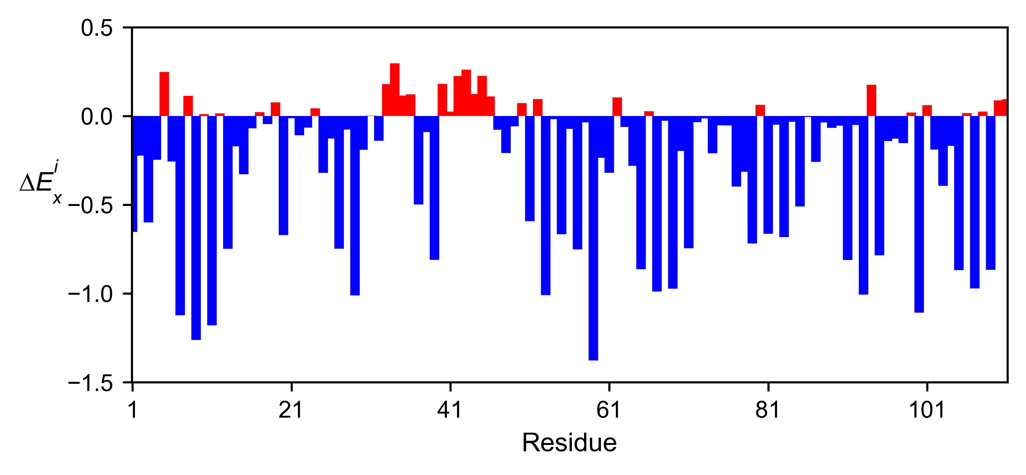
# Positional mean
b11l5f_obj.enrichment_bar(
figsize=[6, 2.5],
mode='mean',
yscale=[-1.5, 0.5],
title='',
)
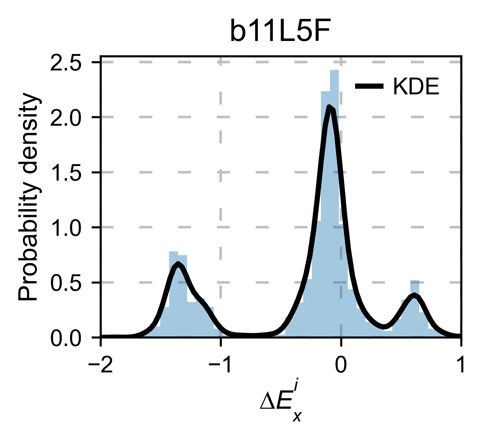
# Kernel
b11l5f_obj.kernel(
histogram=True, title='b11l5f', xscale=[-2, 1], output_file=None
)
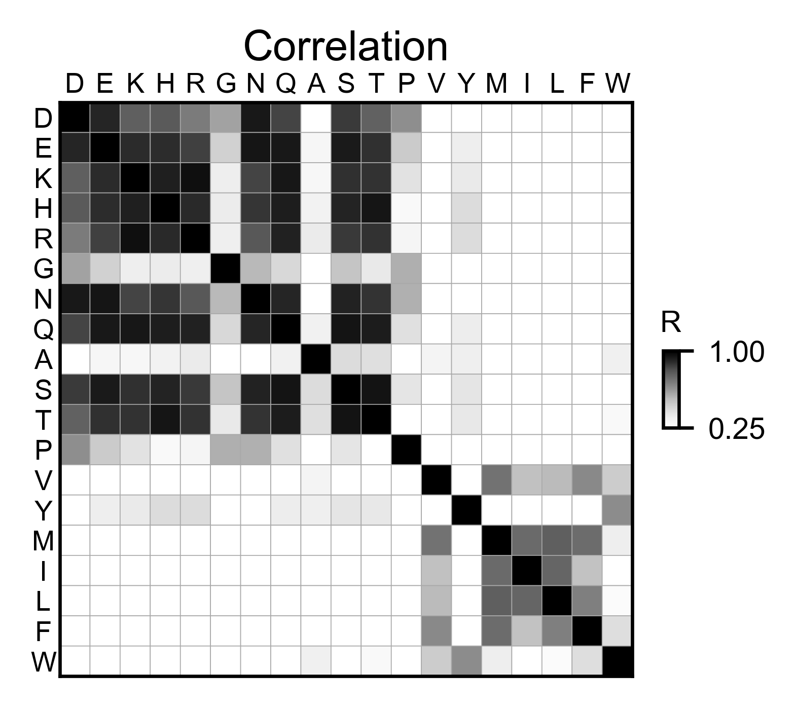
# Correlation between amino acids
b11l5f_obj.correlation(
colorbar_scale=[0.25, 1],
title='Correlation',
neworder_aminoacids=neworder_aminoacids,
)
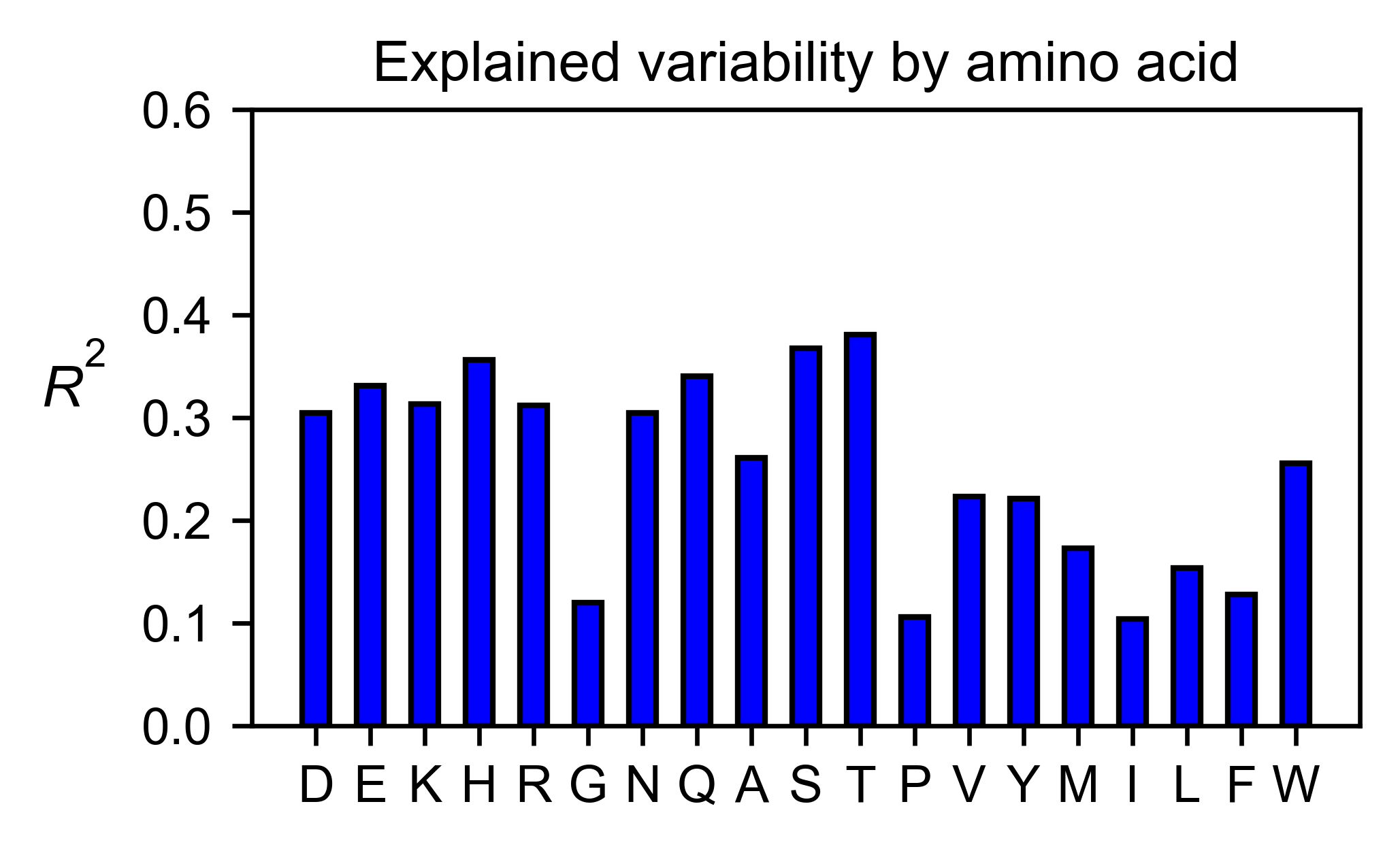
# Explained variability by amino acid
b11l5f_obj.individual_correlation(
yscale=[0, 0.6],
title='Explained variability by amino acid',
neworder_aminoacids=neworder_aminoacids,
)
# PCA by amino acid substitution
b11l5f_obj.pca(
title='',
dimensions=[0, 1],
figsize=(2, 2),
adjustlabels=True,
neworder_aminoacids=neworder_aminoacids,
)
References
The raw data was extracted from published material. Here are the sources: beta lactamase [6] , sumo1 and ube2i [7] , mapk1 [3] , tat and rev [2] , alpha-synuclein [5] , aph(3)II [4] , b11l5f [1] ).
| [1] | Dou, J., Vorobieva, A., Sheffler, W., Doyle, L., Park, H., Bick, M., … Baker, D. (2018). De Novo Design Of A Fluorescence-Activating Β-Barrel. Zenodo. doi:10.5281/zenodo.1216229 |
| [2] | Fernandes, J. D., Faust, T. B., Strauli, N. B., Smith, C., Crosby, D. C., Nakamura, R. L., … Frankel, A. D. (2016). Functional segregation of overlapping genes in HIV. Cell, 167(7), 1762–1773.e12. doi:10.1016/j.cell.2016.11.031 |
| [3] | Livesey, B. J., & Marsh, J. A. (2020). Using deep mutational scanning to benchmark variant effect predictors and identify disease mutations. Molecular Systems Biology, 16(7), e9380. doi:10.15252/msb.20199380 |
| [4] | Melnikov, A., Rogov, P., Wang, L., Gnirke, A., & Mikkelsen, T. S. (2014). Comprehensive mutational scanning of a kinase in vivo reveals substrate-dependent fitness landscapes. Nucleic Acids Research, 42(14), e112. doi:10.1093/nar/gku511 |
| [5] | Newberry, R. W., Leong, J. T., Chow, E. D., Kampmann, M., & DeGrado, W. F. (2020). Deep mutational scanning reveals the structural basis for α-synuclein activity. Nature Chemical Biology, 16(6), 653–659. doi:10.1038/s41589-020-0480-6 |
| [6] | Stiffler, M. A., Hekstra, D. R., & Ranganathan, R. (2015). Evolvability as a function of purifying selection in TEM-1 β-lactamase. Cell, 160(5), 882–892. doi:10.1016/j.cell.2015.01.035 |
| [7] | Weile, J., Sun, S., Cote, A. G., Knapp, J., Verby, M., Mellor, J. C., … Roth, F. P. (2017). A framework for exhaustively mapping functional missense variants. Molecular Systems Biology, 13(12), 957. doi:10.15252/msb.20177908 |