Tutorial introduction

Let’s take a look to the workflow:

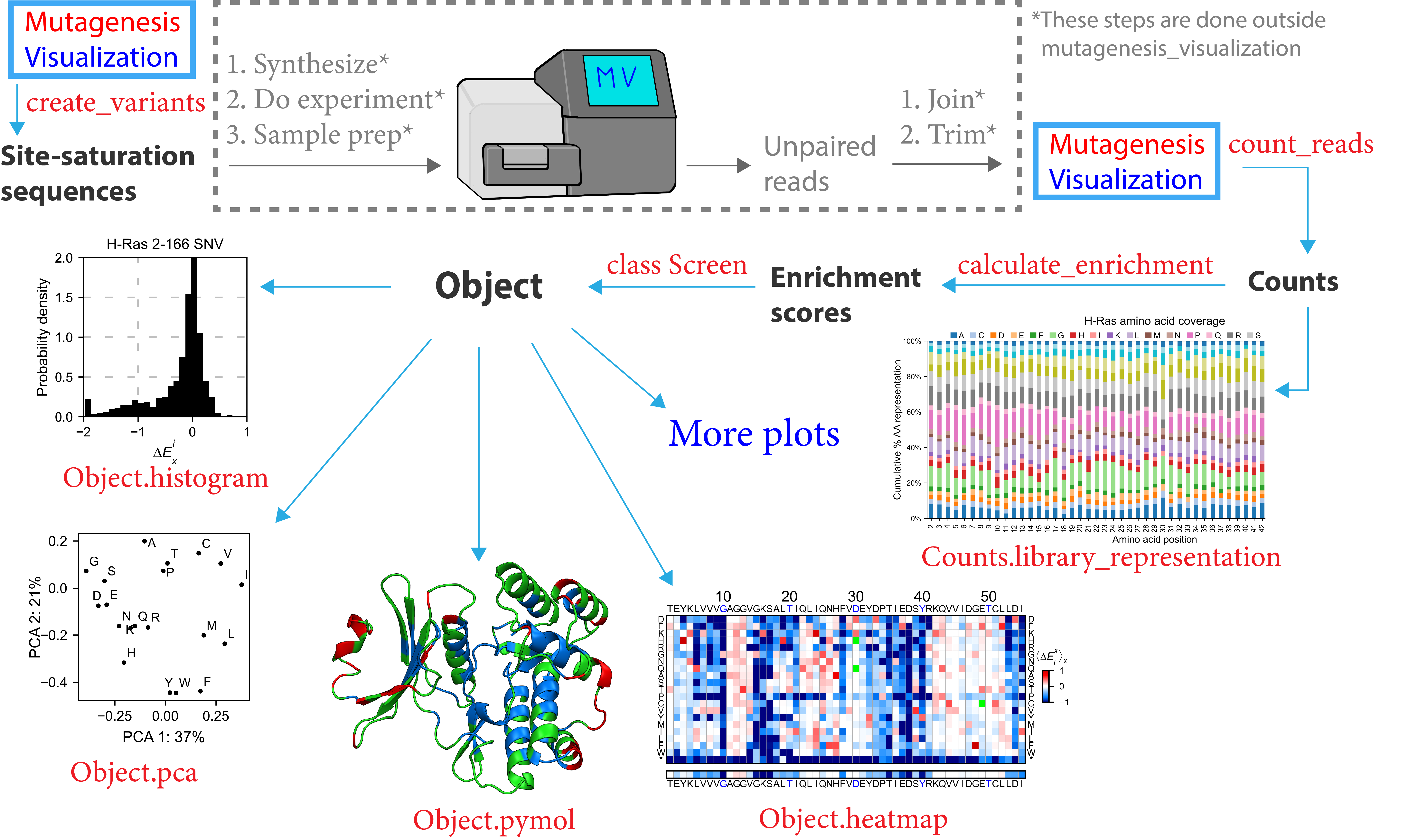
To start, you can use this software to design site-saturation sequences (doc1_library.ipynb). From here, you will pause your work with Mutagenesis_visualization to synthesize the site-saturation sequences using Twist Bio, Agilent, etc. Once you have got your DNA library ready, you will perform the necessary experiments and sequence the samples. After that, you will use a bioinformatics software (ie Flash) to pair the unpaired reads. Then you will trim the adapters to generate FASTQ files.

Now you will return to the software to conduct the data processing of your experiment (doc2_processing.ipynb). Mutagenesis_visualization will read the FASTQ files and return the counts per variant. At this point, there are a few visualization plots that you can create in order to assess the quality of the DNA library. After that, you will calculate the enrichment scores using the calculate_enrichment function (you will need a pre-selection and a post-selection dataset). There are different ways of conducting the data normalization, and you should see what parameters fit your interests best (doc3_normalizing.ipynb).

With the enrichment scores in hand, you will have multiple options to plot and visualize the data, including heatmaps, histograms, scatter plots, PCA analysis, Pymol figures, and more (doc4a_heatmaps.ipynb and doc4b_plotting.ipynb) and (doc5_plotly.ipynb). We have compiled other people’s datasets and visualized them (doc6_other_datasets.ipynb).

You can access the jupyter notebooks and play with the code in mybinder.