Processing DNA reads
This section will teach you how to use the built-in data muting functions. If you already have your own muting pipeline built, you can skip this section and go to the plotting examples.
Import module
%matplotlib inline
from typing import List
import numpy as np
import pandas as pd
from pandas.core.frame import DataFrame
from mutagenesis_visualization import count_reads
from mutagenesis_visualization import count_fastq
from mutagenesis_visualization import calculate_enrichment

from mutagenesis_visualization.main.utils.data_paths import HRAS_FASTQ, HRAS_GAPGEF_COUNTS
from mutagenesis_visualization import Counts
from mutagenesis_visualization import Screen
Count DNA reads from fastq file
Site saturation mutagenesis
- Methods and functions reviewed in this notebook:
After sequencing your DNA library, using other packages you will
assemble the forward and reverse reads and trim the flanking bases. That
will produce a trimmed fastq file that contains the DNA reads. This is
where mutagenesis_visualization kicks in. The following function
count_reads will read your trimmed fastq file and count the number
of times a DNA sequence is present. You will have to pass as inputs a
dna_sequence and a codon_list with the codons that were used to
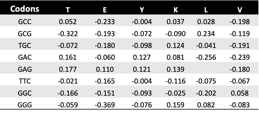
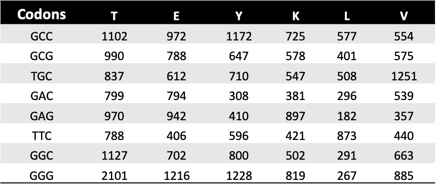
make the point mutant library. If savefile=True , it will export the
results to txt files. Below there is a prettified example of the output
file.
# H-Ras dna sequence
hras_dnasequence: str = 'acggaatataagctggtggtggtgggcgccggcggtgtgggcaagagtgcgctgaccat'\
    + 'ccagctgatccagaaccattttgtggacgaatacgaccccactatagaggattcctaccggaagcaggtgg'\
    + 'tcattgatggggagacgtgcctgttggacatcctg'

# Codons used to make the NNS library. I could also have used 'NNS' and the package will use the NNS codons
codon_list: List[str] = [
    "GCC", "GCG", "TGC", "GAC", "GAG", "TTC", "GGC", "GGG", "CAC", "ATC", "AAG",
    "CTC", "CTG", "TTG", "ATG", "AAC", "CCC", "CCG", "CAG", "CGC", "CGG", "AGG",
    "TCC", "TCG", "AGC", "ACC", "ACG", "GTC", "GTG", "TGG", "TAC", "TAG"
]

counts_wt: bool = False
start_position: int = 2

# Execute count reads
df_counts_pre, wt_counts_pre = count_reads(
    hras_dnasequence, HRAS_FASTQ, codon_list, counts_wt, start_position)
Create object of class Counts.
hras_obj = Counts(df_counts_pre, start_position = 2)
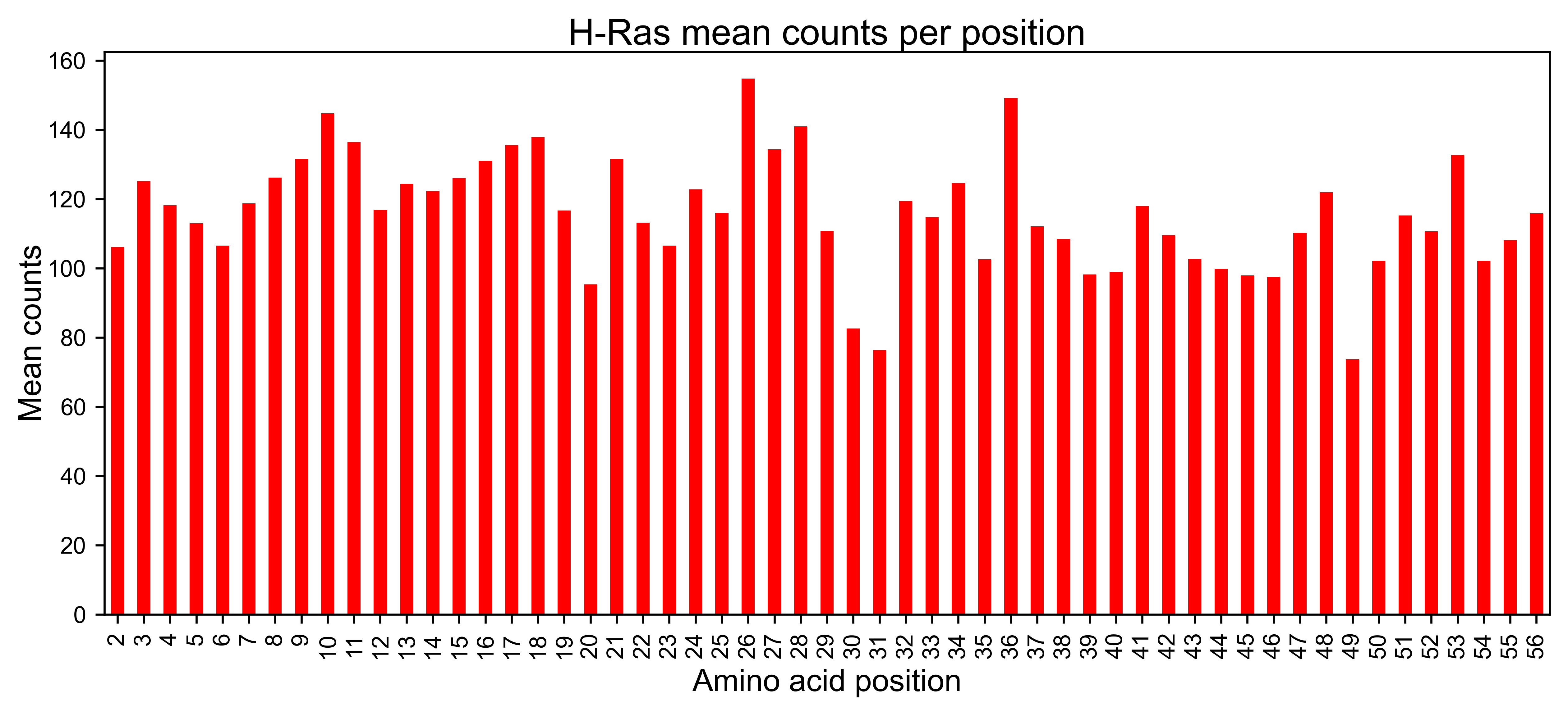
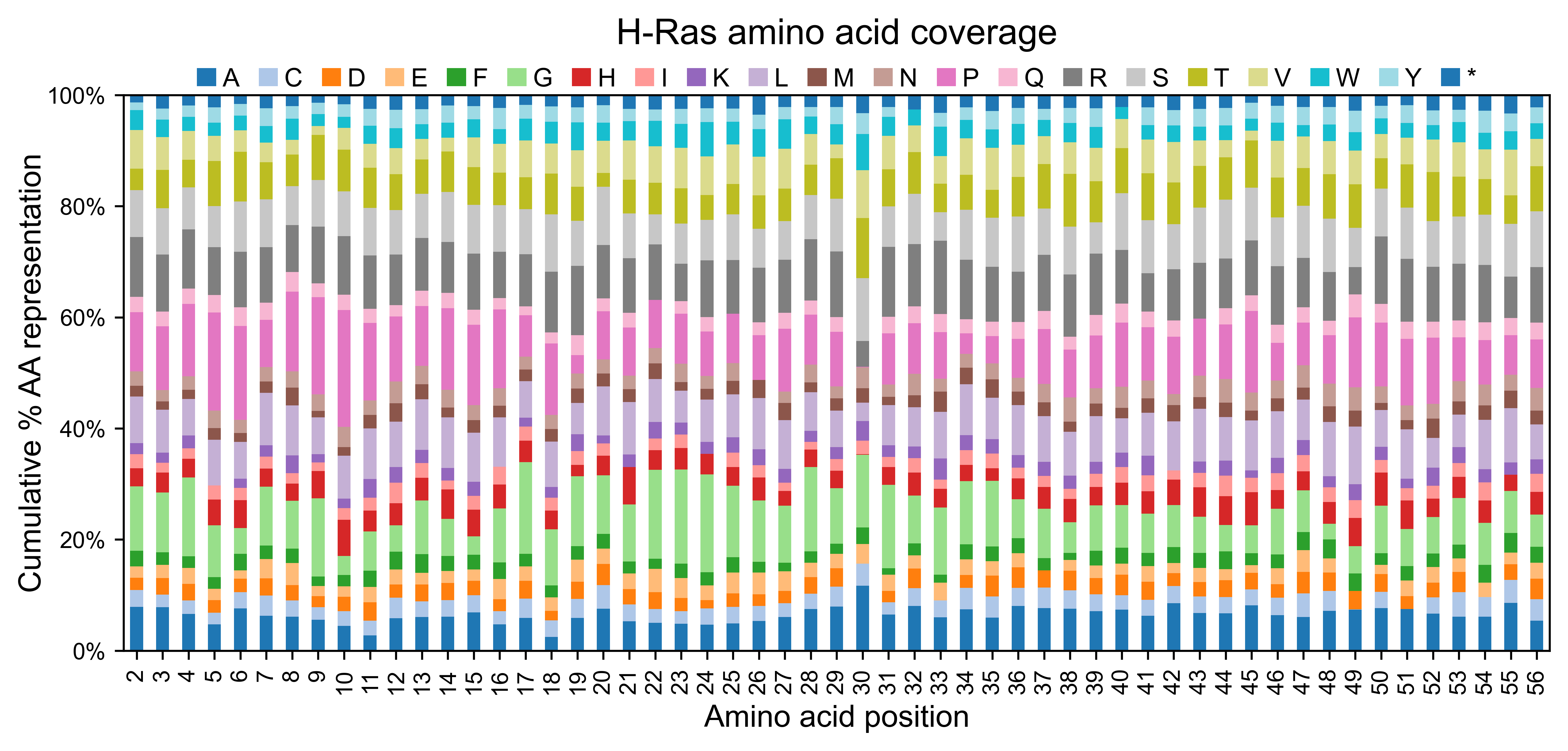
Once the reads have been counted, the method mean_counts can be used
to evaluate the coverage by position. The method
library_representation will tell you the percentage coverage of each
amino acid per position.
hras_obj.mean_counts(title='H-Ras mean counts per position')

hras_obj.library_representation(title='H-Ras amino acid coverage')
Custom DNA list
Use a custom input DNA list. That way it does not matter if you are using NNS or you have second order mutations. Create a list of variants on your own, and the software will count the frequency of each of those variants on the fastq file you provide as an input. In the example non of the sequences we are specifying are found in the trimmed file, thus there are 0% of useful reads.
# Create your list of variants
variants: List[str] = [
    'acggaatataagctggtggtggtgggcgccggcggtgtgggcaagagtgcgctgaccat' +
    'ccagctgatccagaaccattttgtggacgaatacgaccccactatagaggattcctaccggaagcaggtgg' +
    'tcattgatggggagacgtgcctgttggacatcctg',
    'aaaaaatataagctggtggtggtgggcgccggcggtgtgggcaagagtgcgctgaccat' +
    'ccagctgatccagaaccattttgtggacgaatacgaccccactatagaggattcctaccggaagcaggtgg' +
    'tcattgatggggagacgtgcctgttggacatcctg',
    'tttttttataagctggtggtggtgggcgccggcggtgtgggcaagagtgcgctgaccat' +
    'ccagctgatccagaaccattttgtggacgaatacgaccccactatagaggattcctaccggaagcaggtgg' +
    'tcattgatggggagacgtgcctgttggacatcctg'
]

variants, totalreads, usefulreads = count_fastq(variants, HRAS_FASTQ)

# Evaluate how many variants in the fastq file were useful
print(
    '{}/{} useful reads ({}%)'.format(
        str(usefulreads), str(totalreads),
        str(int(usefulreads / totalreads * 100))
    )
)
Calculate enrichment scores
- Methods and functions reviewed in this section:
If you are performing a selection experiment, where you sequence your
library before and after selection, you will need to calculate the
enrichment score of each mutant. The function to do so is
calculate_enrichment. This function allows for different parameters
to tune how the data is muted and normalized.
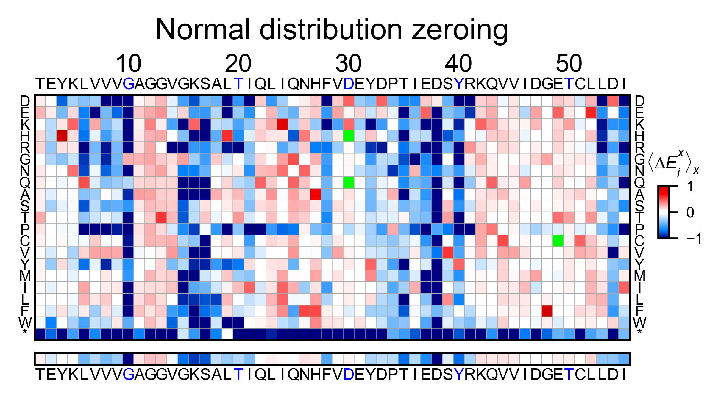
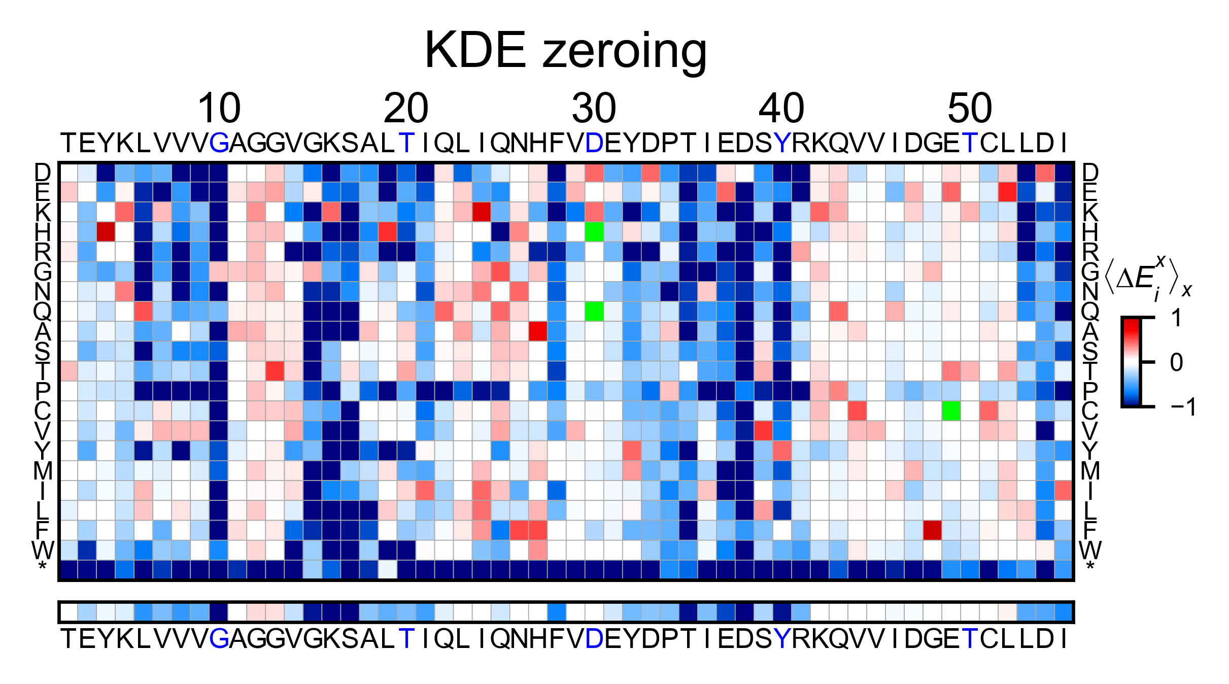
In this example, we show two different ways of using calculate_enrichment. Note that the parameters of choice will have a say on the final result. In the example, the tonality of red of the two heatmaps is slightly different. A more detailed explanation of the parameters can be found in Normalizing datasets.
# Read counts from file (could be txt, csv, xlsx, etc...)
df_counts_pre: DataFrame = pd.read_excel(
    HRAS_GAPGEF_COUNTS,
    'R1_before',
    skiprows=1,
    index_col='Codons',
    usecols='E:FN',
    nrows=32
)

df_counts_sel: DataFrame = pd.read_excel(
    HRAS_GAPGEF_COUNTS,
    'R1_after',
    skiprows=1,
    index_col='Codons',
    usecols='E:FN',
    nrows=32
)
# Ras parameters to create an object

# Define protein sequence
hras_sequence: str = 'MTEYKLVVVGAGGVGKSALTIQLIQNHFVDEYDPTIEDSYRKQVVIDGETCLLDILDTAGQEEY'\
                + 'SAMRDQYMRTGEGFLCVFAINNTKSFEDIHQYREQIKRVKDSDDVPMVLVGNKCDLAARTVES'\
                + 'RQAQDLARSYGIPYIETSAKTRQGVEDAFYTLVREIRQHKLRKLNPPDESGPG'

# Order of amino acid substitutions in the hras_enrichment dataset
aminoacids: List[str] = list('ACDEFGHIKLMNPQRSTVWY*')

# First residue of the hras_enrichment dataset. Because 1-Met was not mutated, the dataset starts at residue 2
start_position: int = 2

# Define secondary structure
secondary = [['L0'], ['β1'] * (9 - 1), ['L1'] * (15 - 9), ['α1'] * (25 - 15),
             ['L2'] * (36 - 25), ['β2'] * (46 - 36), ['L3'] * (48 - 46),
             ['β3'] * (58 - 48), ['L4'] * (64 - 58), ['α2'] * (74 - 64),
             ['L5'] * (76 - 74), ['β4'] * (83 - 76), ['L6'] * (86 - 83),
             ['α3'] * (103 - 86), ['L7'] * (110 - 103), ['β5'] * (116 - 110),
             ['L8'] * (126 - 116), ['α4'] * (137 - 126), ['L9'] * (140 - 137),
             ['β6'] * (143 - 140), ['L10'] * (151 - 143), ['α5'] * (172 - 151),
             ['L11'] * (190 - 172)]

# Substitute Nan values with 0
fillna = 0
# Order of amino acids (from count_reads)
aminoacids_NNS: List[str] = list('AACDEFGGHIKLLLMNPPQRRRSSSTTVVWY*')

# Different parameters can be used to calculate the enrichment scores. They are described in the implementation section

# Zeroing using the median of the population, and not using stop codons to correct.
frequencies = calculate_enrichment(
    aminoacids=aminoacids_NNS,
    pre_lib=df_counts_pre.iloc[:, :54],
    post_lib=df_counts_sel.iloc[:, :54],
    zeroing_method='population',
    zeroing_metric ='median',
    norm_std=True,
    stopcodon=True,
    min_counts=25,
    min_countswt=100,
    mpop=2,
    mwt=2,
    infinite=3,
    std_scale=0.3
)

hras_example1 = Screen(
    np.array(frequencies), hras_sequence, aminoacids, start_position, fillna,
    secondary
)

hras_example1.heatmap(title='Normal distribution zeroing', output_file=None)

# Zeroing using the median of the population, and not using stop codons to correct.
frequencies = calculate_enrichment(
    aminoacids=aminoacids_NNS,
    pre_lib=df_counts_pre.iloc[:, :54],
    post_lib=df_counts_sel.iloc[:, :54],
    zeroing_method='kernel',
    zeroing_metric ='median',
    norm_std=True,
    stopcodon=True,
    min_counts=25,
    min_countswt=100,
    mpop=2,
    mwt=2,
    infinite=3,
    std_scale=0.15
)

hras_example2 = Screen(
    np.array(frequencies), hras_sequence, aminoacids, start_position, fillna,
    secondary
)

hras_example2.heatmap(title='KDE zeroing', output_file=None)

# Note that the two heatmaps look quite similar but the red tonality is slighly different. That is caused by
# small differences in zeroing the data.