Normalizing datasets
This section will teach the different options to normalize the data using the function mutagenesis_visualization.calculate_enrichment() .
If you already have your own processing pipeline built, you can skip this section and go to the (Creating plots) examples.
Import modules and load data
%matplotlib inline
from typing import List, Dict
import numpy as np
import pandas as pd
from pandas.core.frame import DataFrame

from mutagenesis_visualization import calculate_enrichment
from mutagenesis_visualization.main.utils.data_paths import HRAS_RBD_COUNTS
from mutagenesis_visualization import Screen
Now let’s add some information about Ras.
# Define protein sequence
hras_sequence: str = 'MTEYKLVVVGAGGVGKSALTIQLIQNHFVDEYDPTIEDSYRKQVVIDGETCLLDILDTAGQEEY'\
                + 'SAMRDQYMRTGEGFLCVFAINNTKSFEDIHQYREQIKRVKDSDDVPMVLVGNKCDLAARTVES'\
                + 'RQAQDLARSYGIPYIETSAKTRQGVEDAFYTLVREIRQHKLRKLNPPDESGPG'


# First residue of the hras_enrichment dataset. Because 1-Met was not mutated, the dataset starts at residue 2
start_position: int = 2

# Substitute Nan values with 0
fillna: int = 0
# List of sheets and columns to use
sheets_pre: List[str] = ['R1_before', 'R2_before', 'R3_before']
sheets_sel: List[str] = ['R1_after', 'R2_after', 'R3_after']
columns: List[str] = ['F:BG', 'BH:DK', 'DL:FN']
columns_wt: List[str] = ['A', 'B', 'C']

# Create dictionary with data. Loading 3 replicates, each of them is divided into 3 pools
dict_pre, dict_sel, dict_pre_wt, dict_sel_wt = ({} for i in range(4))

# Read counts from file (could be txt, csv, xlsx, etc...)
for column, column_wt in zip(columns, columns_wt):
    for sheet_pre, sheet_sel in zip(sheets_pre, sheets_sel):
        # Pre counts
        label_pre = str(sheet_pre + '_' + column_wt)
        dict_pre[label_pre] = pd.read_excel(
            HRAS_RBD_COUNTS, sheet_pre, skiprows=1, usecols=column, nrows=32
        )
        # Pre counts wild-type alleles
        dict_pre_wt[label_pre] = pd.read_excel(
            HRAS_RBD_COUNTS, sheet_pre, usecols=column_wt
        )

        # Sel counts
        label_sel = str(sheet_sel + '_' + column_wt)
        dict_sel[label_sel] = pd.read_excel(
            HRAS_RBD_COUNTS, sheet_sel, skiprows=1, usecols=column, nrows=32
        )
        # Sel counts wild-type alleles
        dict_sel_wt[label_sel] = pd.read_excel(
            HRAS_RBD_COUNTS, sheet_sel, usecols=column_wt
        )
Calculate log10 enrichment
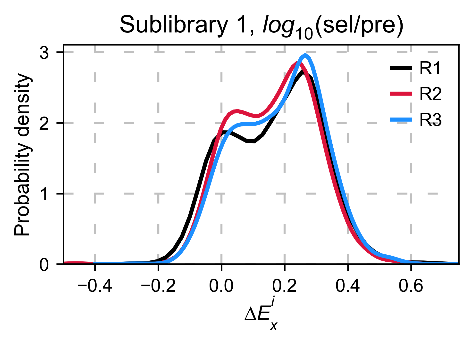
Now we are going to calculate the log10(sel/pre) for the sublibrary 1 of each replicate and plot a histogram. The resulting distribution is bimodal, and because the three replicates have a similar number of counts ratios, their center is overlapping. However, because we have not normalized by the number of counts, and there are more counts in the selected than in the pre-selected population, the center is >0.
# Auxiliar function to convert +-inf values to an arbitrary number (ie +-2)
def _replace_inf(df: DataFrame) -> DataFrame:
    df.replace(to_replace=np.inf, value=2, inplace=True)
    df.replace(to_replace=-np.inf, value=-2, inplace=True)
    return df


aminoacids: List[str] = list('AACDEFGGHIKLLLMNPPQRRRSSSTTVVWY*')
enrichment = {}

# calculate log10 enrichment for each replicate
for pre_key, sel_key in zip(list(dict_pre.keys())[:3],
                            list(dict_sel.keys())[:3]):
    # log 10
    enrichment_log10 = (np.log10(dict_sel[sel_key] / dict_pre[pre_key]))
    enrichment_log10['aminoacids'] = aminoacids
    enrichment_log10.set_index(['aminoacids'], inplace=True)
    enrichment[pre_key[:2]] = _replace_inf(enrichment_log10)

# Create objects
hras_object: Screen = Screen(
    list(enrichment.values()), hras_sequence, aminoacids, start_position, fillna,
)

hras_object.kernel(show_replicates=True, kernel_color_replicates = ["b", "r", "g"], title=r'$log_{10}$' + '(sel/pre)', xscale=(-1, 1))
Centering the data (zeroing)
- Functions used in this section:
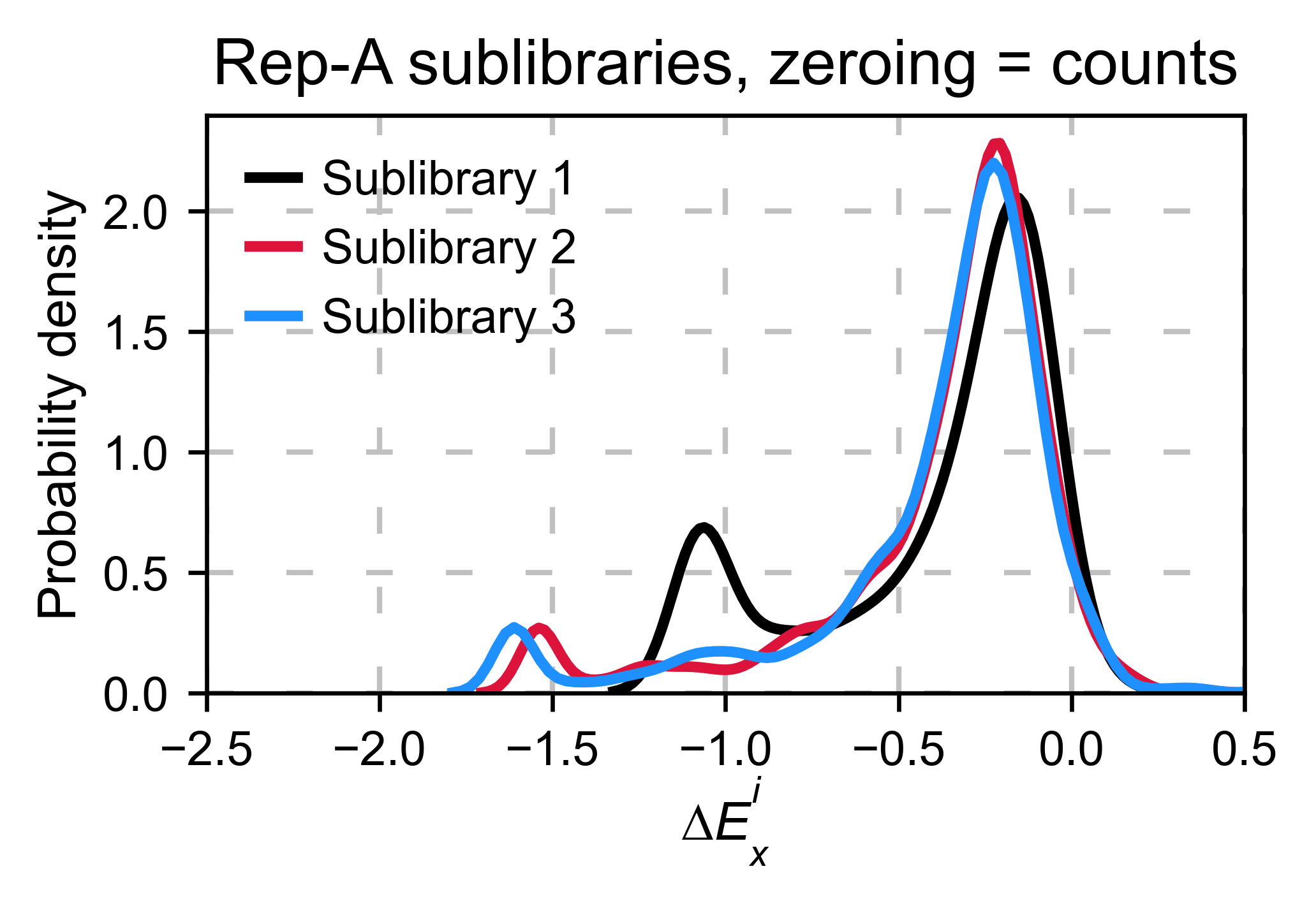
Counts normalization
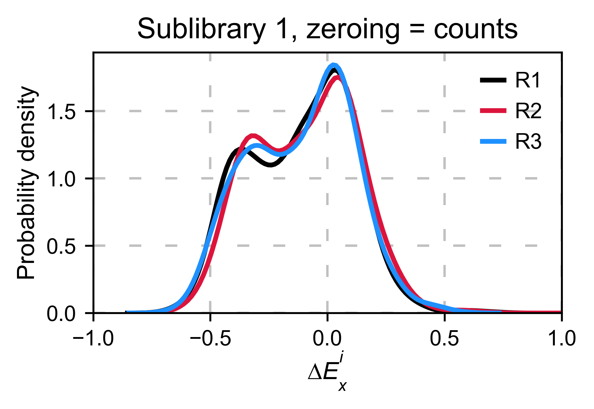
Normalizing by the number of counts improves normalization. Now the
population center is closer to 0. To do so, set
zeroing_method='counts'.
enrichment = {}
aminoacids: List[str] = list('AACDEFGGHIKLLLMNPPQRRRSSSTTVVWY*')
# calculate log10 enrichment for each replicate
for pre_key, sel_key in zip(list(dict_pre.keys())[:3],
                            list(dict_sel.keys())[:3]):
    # Enrichment
    enrichment[pre_key[:2]] = calculate_enrichment(
        aminoacids, dict_pre[pre_key], dict_sel[sel_key], zeroing_method='counts', stopcodon=False
    )

# Plot histogram and KDE
aminoacids: List[str] = list('ACDEFGHIKLMNPQRSTVWY*')

hras_object: Screen = Screen(
    list(enrichment.values()), hras_sequence, aminoacids, start_position, fillna,
)

hras_object.kernel(show_replicates=True, kernel_color_replicates = ["b", "r", "g"], title='zeroing_method = counts', xscale=(-1, 0.5))
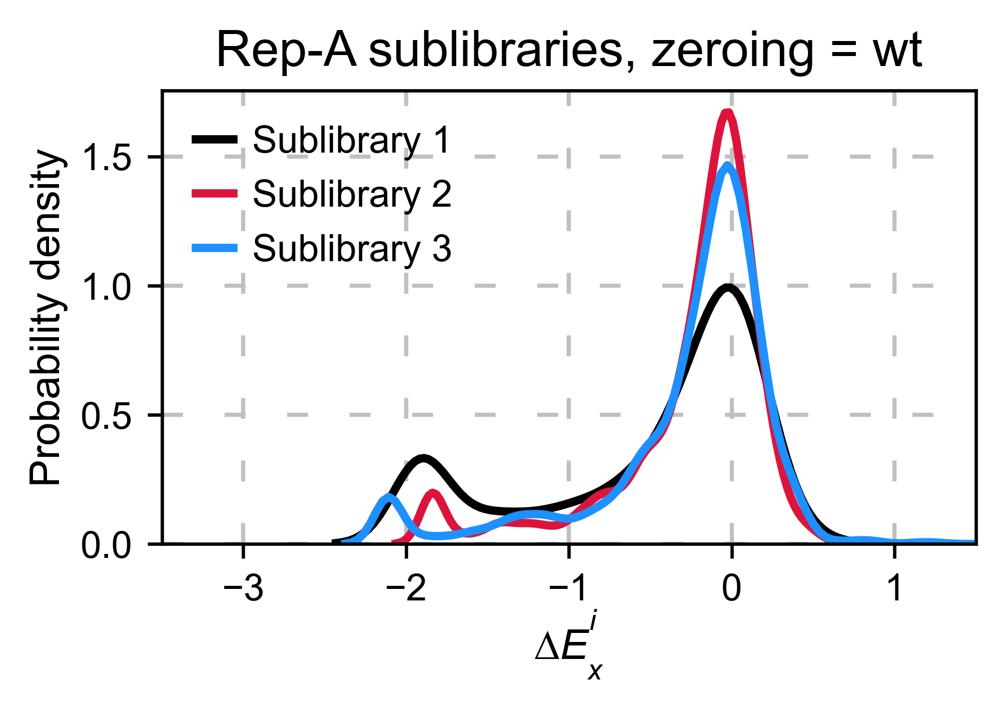
Wt allele
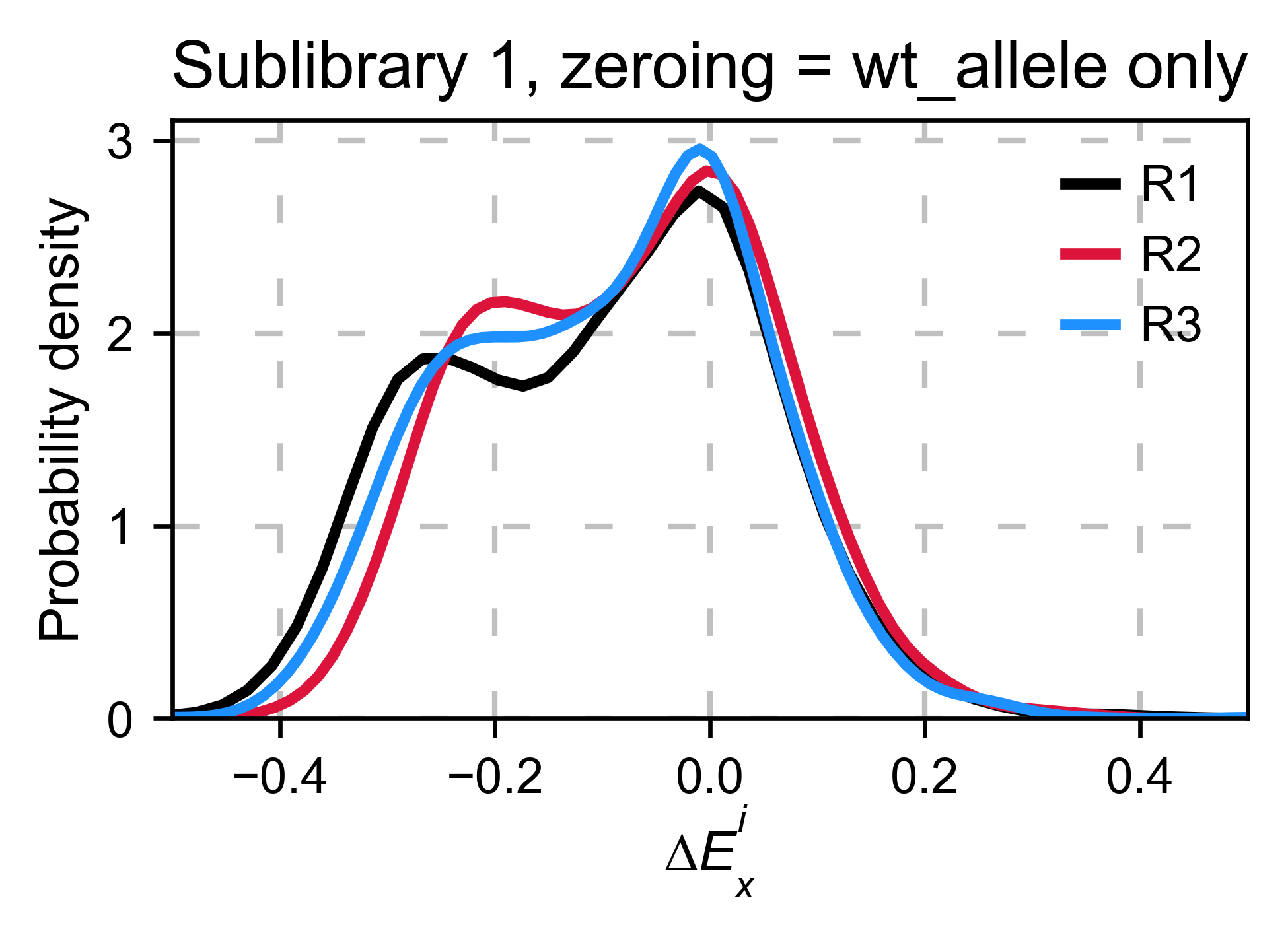
Another way we can normalize is by using an internal reference such as a particular mutant. In the following example we will use the wild-type allele. If the assay that you are using is noisy, relying on a single data point for normalizing will result in high variance. The package does not include this option because it may lead to errors. Here we are showing how it would be done by hand. In this example, it works fine. But in other datasets we have, it has been a source of error.
# calculate log10 enrichment for each replicate

aminoacids: List[str] = list('AACDEFGGHIKLLLMNPPQRRRSSSTTVVWY*')
enrichment = {}

# calculate log10 enrichment for each replicate
for pre_key, sel_key in zip(list(dict_pre.keys())[:3],
                            list(dict_sel.keys())[:3]):
    # log 10
    wt_ratio = np.log10(
        dict_sel_wt[sel_key]['wt 2-56'][1] / dict_pre_wt[pre_key]['wt 2-56'][1]
    )
    enrichment_log10 = np.log10(
        dict_sel[sel_key] / dict_pre[pre_key]
    ) - wt_ratio
    enrichment_log10['aminoacids'] = aminoacids
    enrichment_log10.set_index(['aminoacids'], inplace=True)
    enrichment[pre_key[:2]] = _replace_inf(enrichment_log10)

hras_object: Screen = Screen(
    list(enrichment.values()), hras_sequence, aminoacids, start_position, fillna,
)
hras_object.kernel(show_replicates=True, kernel_color_replicates = ["b", "r", "g"], title='zeroing_method = wt allele only', xscale=(-0.5, 0.5))
Distribution of synonymous wt alleles
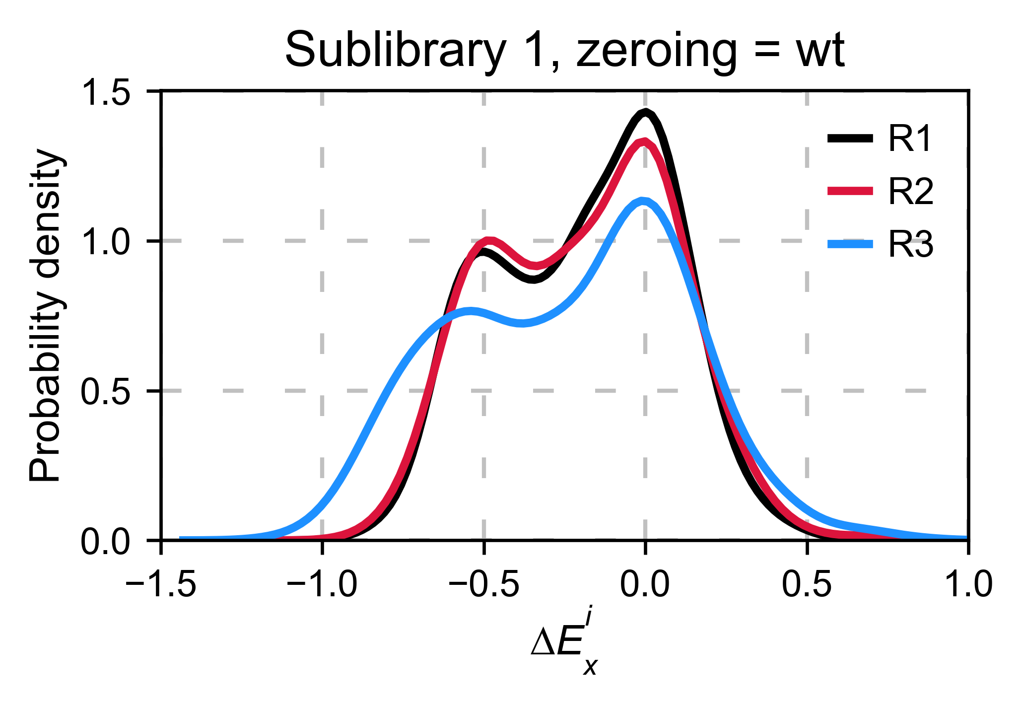
In our experience, it is better to use the median/mode/mean of the
synonymous wild-type population because there is less variance.
calculate_enrichment has such an options by using
zeroing_method='wt' and then
zeroing_metric ='median', 'mean' or 'mode'.
enrichment = {}
aminoacids: List[str] = list('AACDEFGGHIKLLLMNPPQRRRSSSTTVVWY*')

# calculate log10 enrichment for each replicate
for pre_key, sel_key in zip(list(dict_pre.keys())[:3],
                            list(dict_sel.keys())[:3]):
    # Enrichment
    enrichment[pre_key[:2]] = calculate_enrichment(
        aminoacids,
        dict_pre[pre_key],
        dict_sel[sel_key],
        dict_pre_wt[pre_key],
        dict_sel_wt[sel_key],
        zeroing_method='wt',
        zeroing_metric ='mode',
        stopcodon=False
    )

aminoacids: List[str] = list('ACDEFGHIKLMNPQRSTVWY*')

hras_object: Screen = Screen(
    list(enrichment.values()), hras_sequence, aminoacids, start_position, fillna,
)
hras_object.kernel(show_replicates=True, title='Sublibrary 1, zeroing_method = wt', xscale=(-1.5, 1))
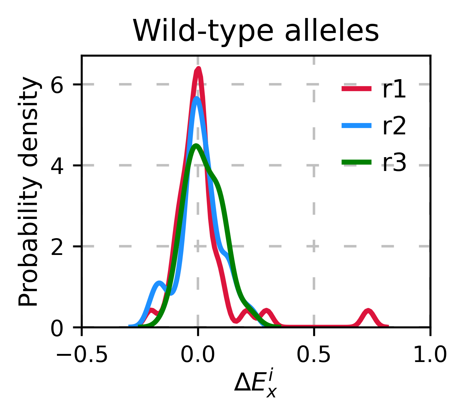
Wt alleles observation
If the population of synonymous wild-type alleles (alleles that are wild-type at a protein level, but not at a DNA level) is small, the distribution of this variants may have high variance from sample to sample. Also, you will notice that not all wild-type alleles are neutral. The spread of these alleles gives a sense of the noise in the experiment.
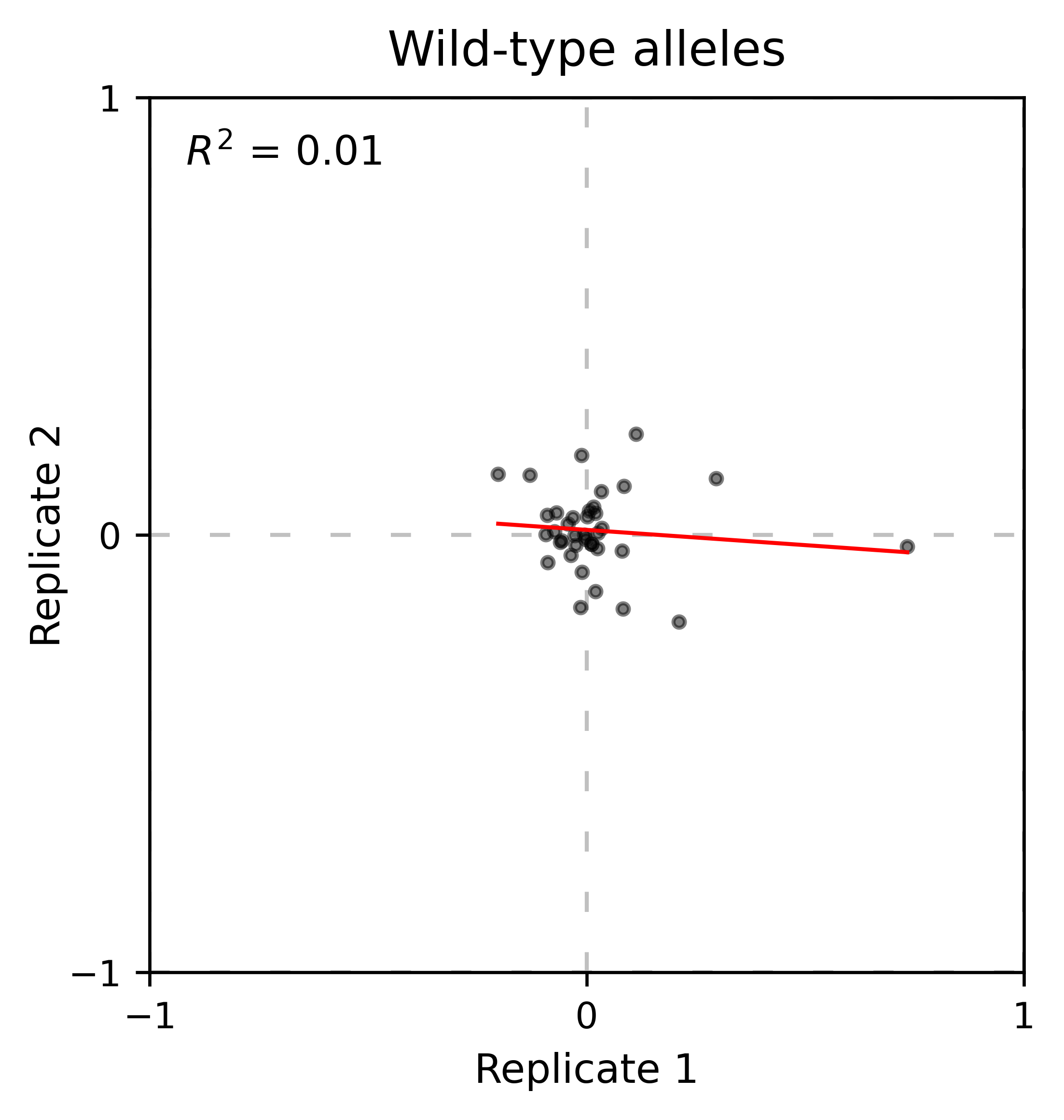
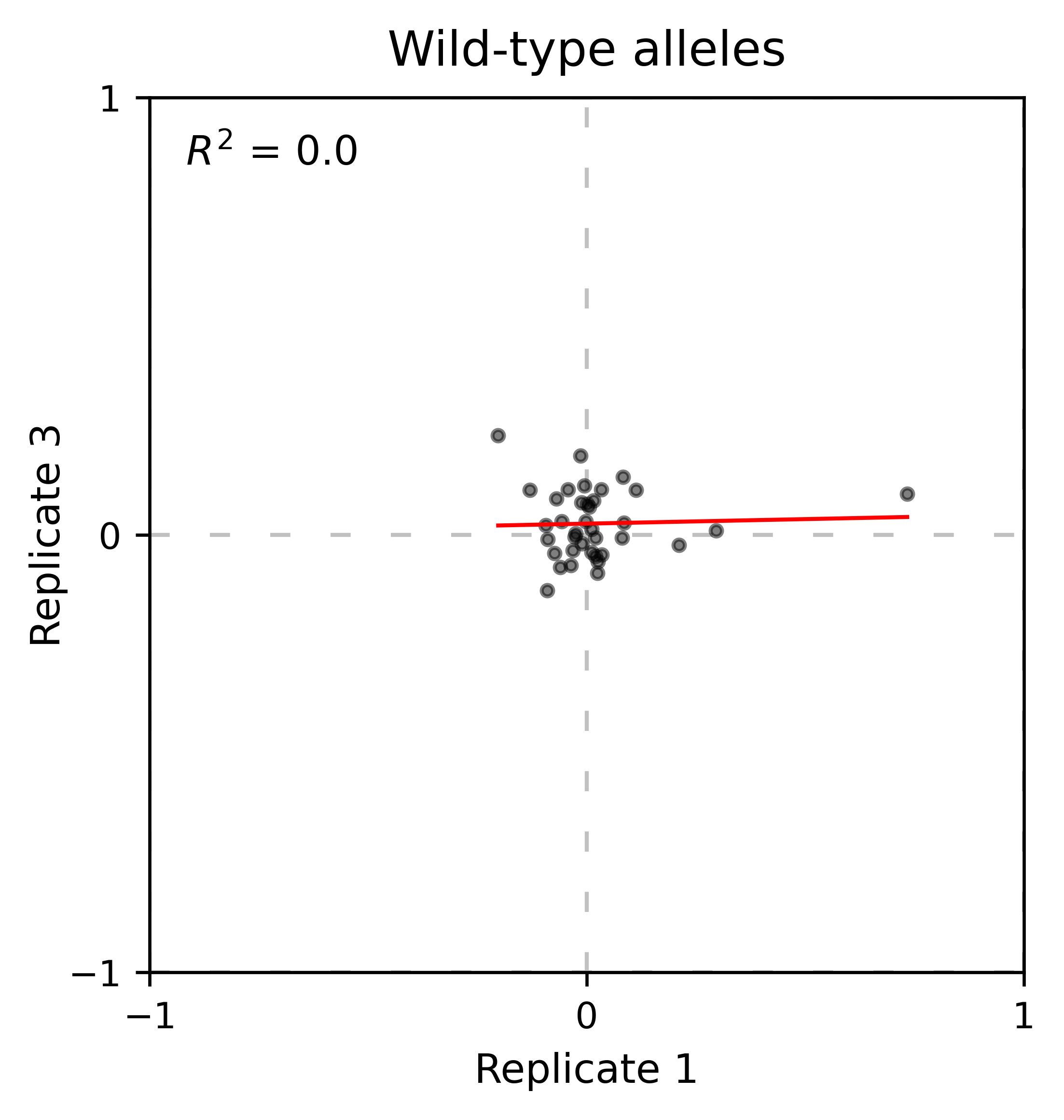
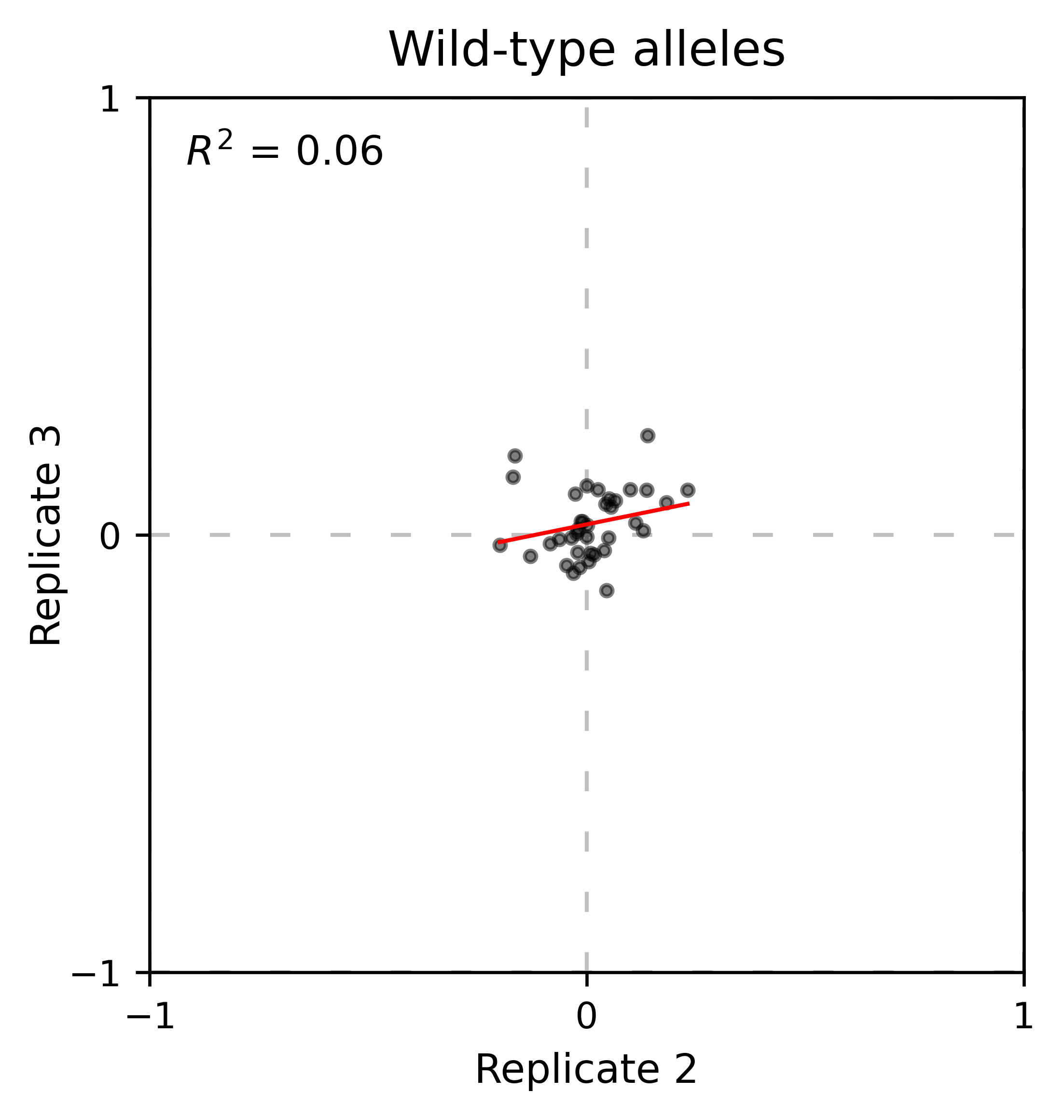
At least for the following data, there is no correlation between the performance of wild-type alleles in different replicates, suggesting that the higher or lower enrichment scores are caused by noise and not a fitness difference caused by changes in protein expression.
hras_object.kernel(show_replicates=True, wt_counts_only=True,title='Wild-type alleles', kernel_colors=['k', 'crimson', 'dodgerblue', 'g', 'silver'], xscale=(-0.5, 1), output_file="docs/images/exported_images/hras_wildtype_distribution.png")
Perform the scatter plots:
hras_object.scatter_replicates(wt_counts_only=True,title='Wild-type alleles', xscale=(-1, 1), yscale=(-1, 1), output_file="docs/images/exported_images/hras_wildtype_scatter.png")
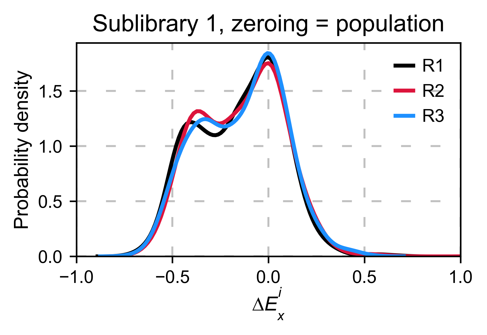
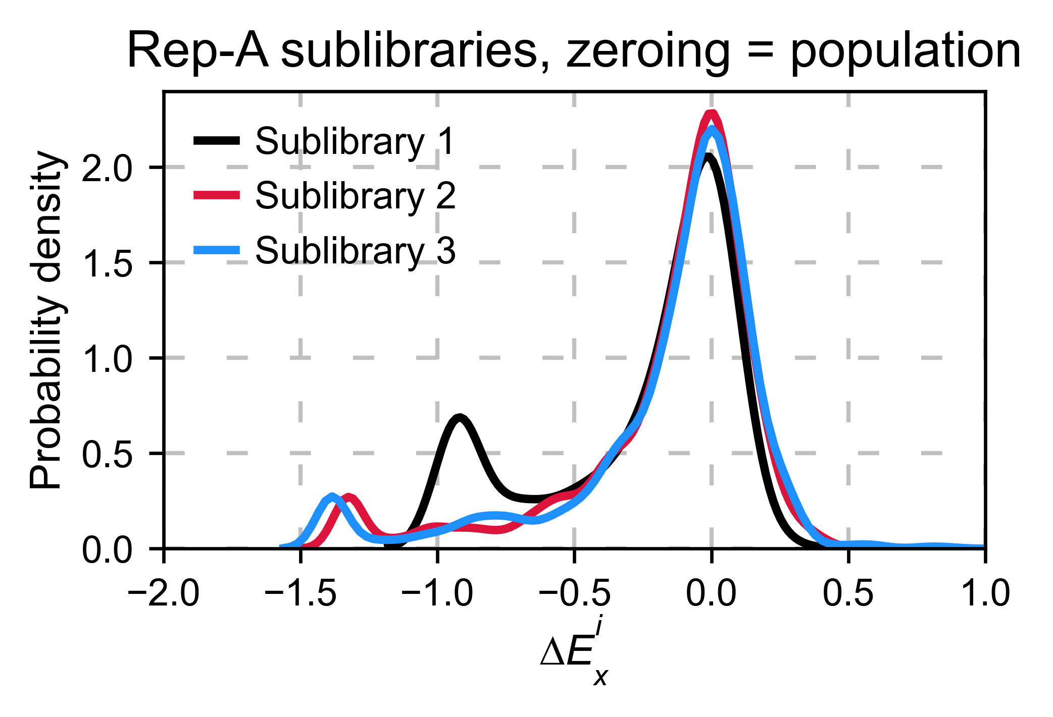
Distribution of mutants
An alternative option to normalize the data is to use the
mean/median/mode of the population to some specific number such as zero.
To do so, use zeroing_method='population'. The parameters of the
distribution will be calculated assuming a gaussian distribution. Not
only the three replicates are centered, but also they have the same
spread.
enrichment = {}
aminoacids: List[str] = list('AACDEFGGHIKLLLMNPPQRRRSSSTTVVWY*')

# calculate log10 enrichment for each replicate
for pre_key, sel_key in zip(list(dict_pre.keys())[:3],
                            list(dict_sel.keys())[:3]):
    # Enrichment
    enrichment[pre_key[:2]]  = calculate_enrichment(
        aminoacids,
        dict_pre[pre_key],
        dict_sel[sel_key],
        zeroing_method='population',
        zeroing_metric ='mode',
        stopcodon=False
    )

aminoacids: List[str] = list('ACDEFGHIKLMNPQRSTVWY*')

hras_object: Screen = Screen(
    list(enrichment.values()), hras_sequence, aminoacids, start_position, fillna,
)
hras_object.kernel(show_replicates=True, title='zeroing_method = population', xscale=(-1, 1))
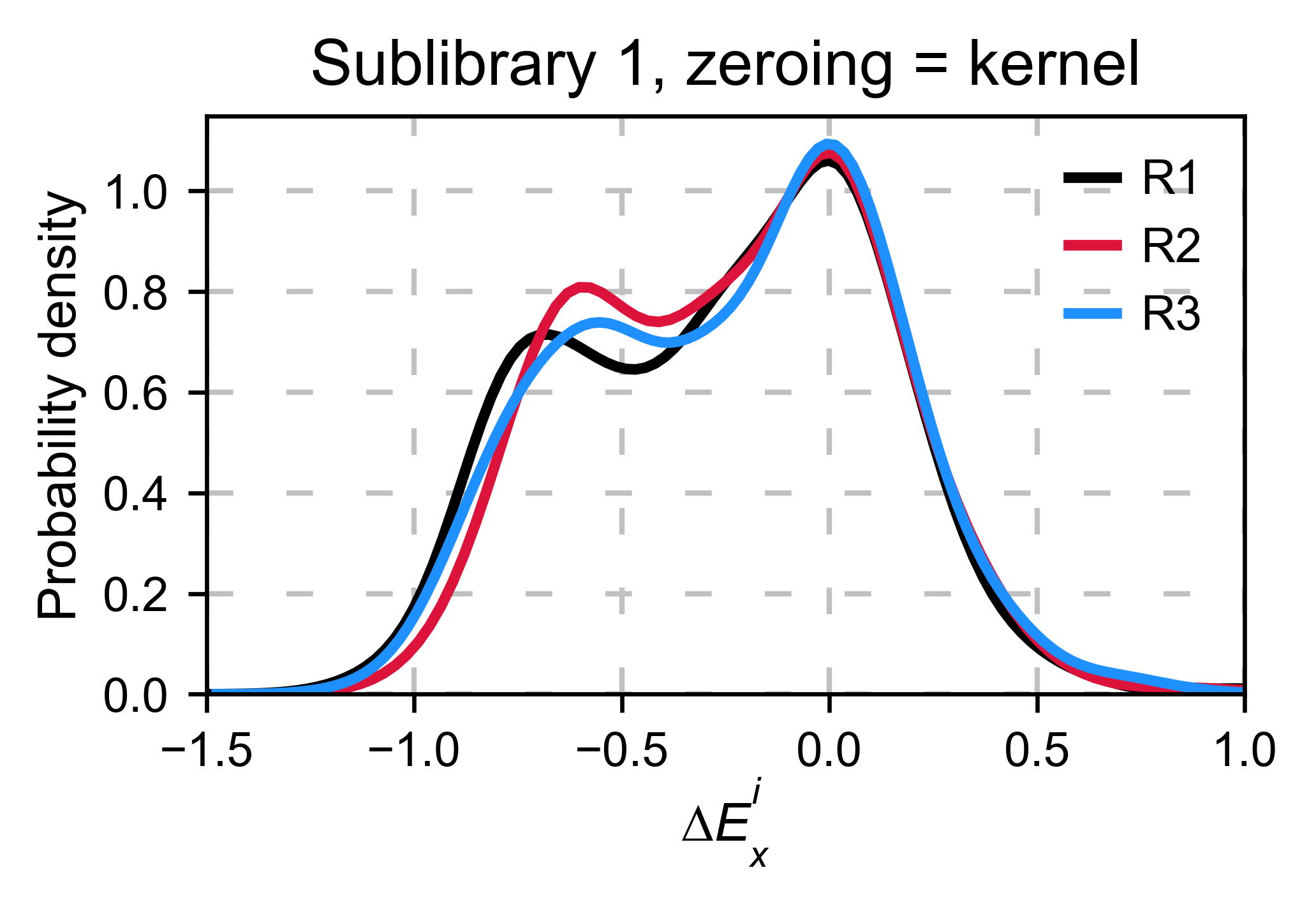
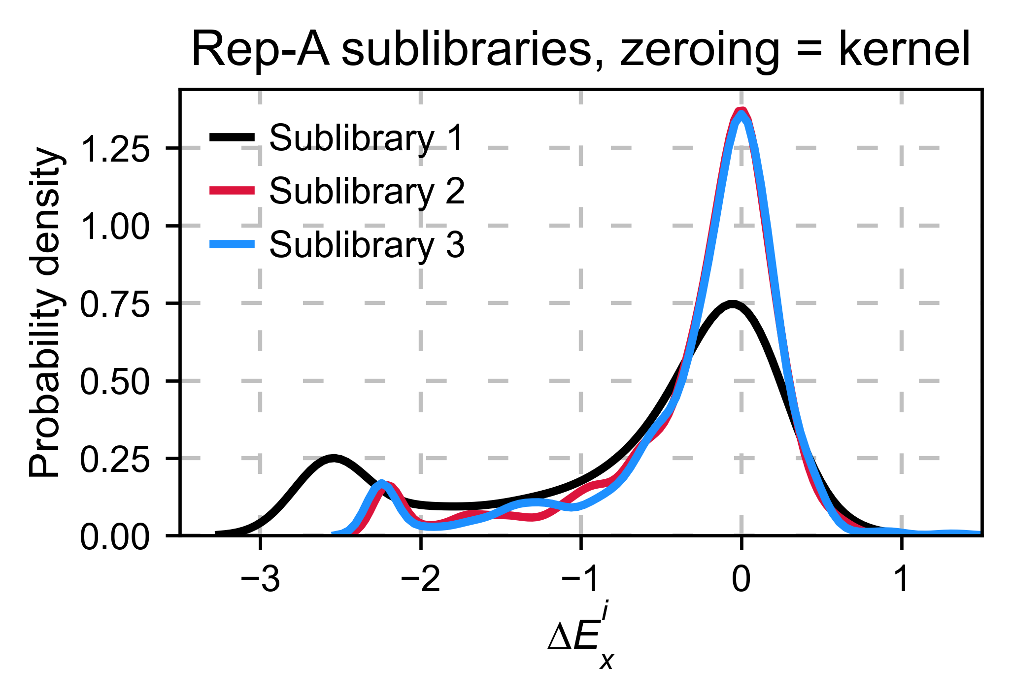
A variant of the previous method is to calculate the kernel density
estimate using zeroing_method='kernel'. This option centers the
population using the mode of the KDE. If the data is bimodal, it will
select the main peak. Furthermore, it will use the standard deviation of
the main peak to scale the data. This method is useful when you have
split your library into multiple pools because it will not only center
the data properly but also do scale the data so each pool main peak has
the same standard deviation. Results are quite similar to setting
zeroing_method='population' and zeroing_metric ='mode'.
enrichment = {}
aminoacids: List[str] = list('AACDEFGGHIKLLLMNPPQRRRSSSTTVVWY*')

# calculate log10 enrichment for each replicate
for pre_key, sel_key in zip(list(dict_pre.keys())[:3],
                            list(dict_sel.keys())[:3]):
    # Enrichment
    enrichment[pre_key[:2]] = calculate_enrichment(
        aminoacids, dict_pre[pre_key], dict_sel[sel_key], zeroing_method='kernel', stopcodon=False
    )

aminoacids: List[str] = list('ACDEFGHIKLMNPQRSTVWY*')

hras_object: Screen = Screen(
    list(enrichment.values()), hras_sequence, aminoacids, start_position, fillna,
)
hras_object.kernel(show_replicates=True, kernel_color_replicates = ["b", "r", "g"],  title='zeroing method = kernel', xscale=(-1.5,1))
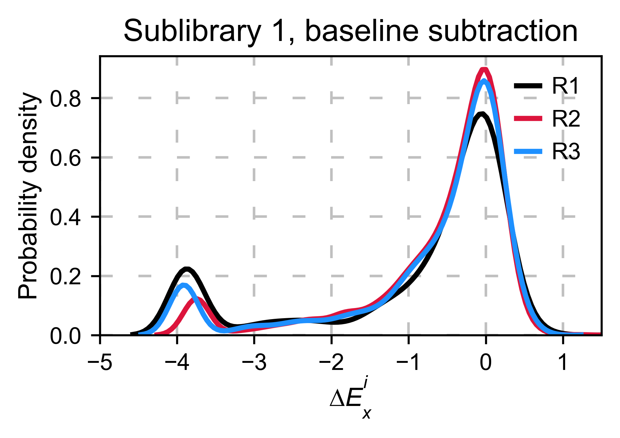
Baseline subtraction
Including stop codons in the library can be of great use because it
gives a control for basal signal in your assay. The algorithm has the
option to apply a baseline subtraction. The way it works is it sets the
stop codons counts of the selected population to 0 (baseline) and
subtracts the the baseline signal to every other mutant. To use this
option, set stopcodon=True. You will notice that it get rids of the
shoulder peak, and now the distribution looks unimodal with a big left
shoulder.
enrichment = {}
aminoacids: List[str] = list('AACDEFGGHIKLLLMNPPQRRRSSSTTVVWY*')

# calculate log10 enrichment for each replicate
for pre_key, sel_key in zip(list(dict_pre.keys())[:3],
                            list(dict_sel.keys())[:3]):
    # Enrichment
    enrichment[pre_key[:2]] = calculate_enrichment(
        aminoacids, dict_pre[pre_key], dict_sel[sel_key], zeroing_method='kernel', stopcodon=True
    )

aminoacids: List[str] = list('ACDEFGHIKLMNPQRSTVWY*')

hras_object: Screen = Screen(
    list(enrichment.values()), hras_sequence, aminoacids, start_position, fillna,
)
hras_object.kernel(show_replicates=True, kernel_color_replicates = ["b", "r", "g"], title='stop codon correction', xscale=(-5, 1.5))
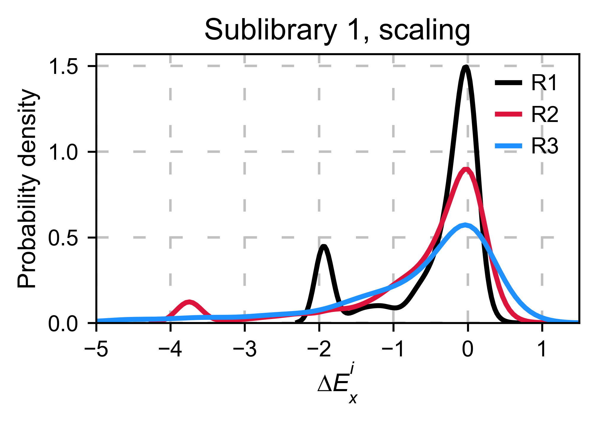
Scaling
By now you probably have realized that different options of
normalization affect to the spread of the data. The rank between each
mutant is unchanged between the different methods, so it is a matter of
multiplying/dividing by a scalar to adjust the data spread. Changing the
value of the parameter std_scale will do the job. You will probably
do some trial an error until you find the right value. In the following
example we are changing the std_scale parameter for each of the
three replicates shown. Note that the higher the scalar, the higher the
spread.
enrichment_scalar = {}
scalars: List[str] = [0.1, 0.2, 0.3]
aminoacids: List[str] = list('AACDEFGGHIKLLLMNPPQRRRSSSTTVVWY*')

# calculate log10 enrichment for each replicate
for pre_key, sel_key, scalar in zip(list(dict_pre.keys())[:3],
                                    list(dict_sel.keys())[:3], scalars):
    # Enrichment
    enrichment_log10 = calculate_enrichment(
        aminoacids,
        dict_pre[pre_key],
        dict_sel[sel_key],
        zeroing_method='kernel',
        stopcodon=True,
        std_scale=scalar
    )
    enrichment_scalar[pre_key[:2]] = enrichment_log10


aminoacids: List[str] = list('ACDEFGHIKLMNPQRSTVWY*')

hras_object: Screen = Screen(
    list(enrichment_scalar.values()), hras_sequence, aminoacids, start_position, fillna,
)
hras_object.kernel(show_replicates=True, kernel_color_replicates = ["b", "r", "g"], title='scaling', xscale=(-5, 1.5))
Multiple sublibraries
In our own research projects, where we have multiple DNA pools, we have
determined that the combination of parameters that best suit us it to
the wild-type synonymous sequences to do a first data normalization
step. Then use zeroing_method = 'kernel' to zero the data and use
stopcodon=True in order to determine the baseline level of signal.
You may need to use different parameters for your purposes. Feel free to
get in touch if you have questions regarding data normalization.
# Labels
labels: List[str] = ['Sublibrary 1', 'Sublibrary 2', 'Sublibrary 3']
zeroing_options: List[str] = ['population', 'counts', 'wt', 'kernel']
title: str = 'Rep-A sublibraries, zeroing_method = '

# xscale
xscales = [(-2, 1), (-2.5, 0.5), (-3.5, 1.5), (-3.5, 1.5)]
# declare dictionary
enrichment_lib = {}
df_lib = {}

for option, xscale in zip(zeroing_options, xscales):
    for pre_key, sel_key, label in zip(list(dict_pre.keys())[::3],
                                       list(dict_sel.keys())[::3], labels):
        aminoacids: List[str] = list('AACDEFGGHIKLLLMNPPQRRRSSSTTVVWY*')

        # log 10
        enrichment_lib[label]  = DataFrame(calculate_enrichment(
            aminoacids,
            dict_pre[pre_key],
            dict_sel[sel_key],
            dict_pre_wt[pre_key],
            dict_sel_wt[sel_key],
            zeroing_method=option,
            zeroing_metric ='mode',
            stopcodon=True,
            infinite=2
        ))

    # Concatenate sublibraries and store in dict
    df_lib[option] = pd.concat([
        enrichment_lib['Sublibrary 1'], enrichment_lib['Sublibrary 2'],
        enrichment_lib['Sublibrary 3']
    ],ignore_index=True, axis=1)


    # Plot
    aminoacids: List[str] = list('ACDEFGHIKLMNPQRSTVWY*')

    hras_sublibrary1: Screen = Screen(
        enrichment_lib['Sublibrary 1'], hras_sequence, aminoacids, start_position, fillna,
    )
    hras_sublibrary2: Screen = Screen(
        enrichment_lib['Sublibrary 2'], hras_sequence, aminoacids, start_position, fillna,
    )
    hras_sublibrary3: Screen = Screen(
        enrichment_lib['Sublibrary 3'], hras_sequence, aminoacids, start_position, fillna,
    )
    hras_sublibrary1.multiple_kernel([hras_sublibrary2, hras_sublibrary3], label_kernels = labels, title=title + option, xscale=xscale)
Heatmaps
- Function and class used in this section:
We are going to evaluate how does the heatmap of produced by each of the
normalization methods. We are not going to scale the data, so some
heatmaps may look more washed out than others. That is not an issue
since can easily be changed by using std_scale.
# First we need to create the objects

# Define protein sequence
hras_sequence: str = 'MTEYKLVVVGAGGVGKSALTIQLIQNHFVDEYDPTIEDSYRKQVVIDGETCLLDILDTAGQEEY'\
                + 'SAMRDQYMRTGEGFLCVFAINNTKSFEDIHQYREQIKRVKDSDDVPMVLVGNKCDLAARTVES'\
                + 'RQAQDLARSYGIPYIETSAKTRQGVEDAFYTLVREIRQHKLRKLNPPDESGPG'

# Order of amino acid substitutions in the hras_enrichment dataset
aminoacids: List[str] = list('ACDEFGHIKLMNPQRSTVWY*')

# First residue of the hras_enrichment dataset. Because 1-Met was not mutated, the dataset starts at residue 2
start_position: int = 2

# Create objects
objects: Dict[str, Screen] = {}
for key, value in df_lib.items():
    temp = Screen(value, hras_sequence, aminoacids, start_position)
    objects[key] = temp
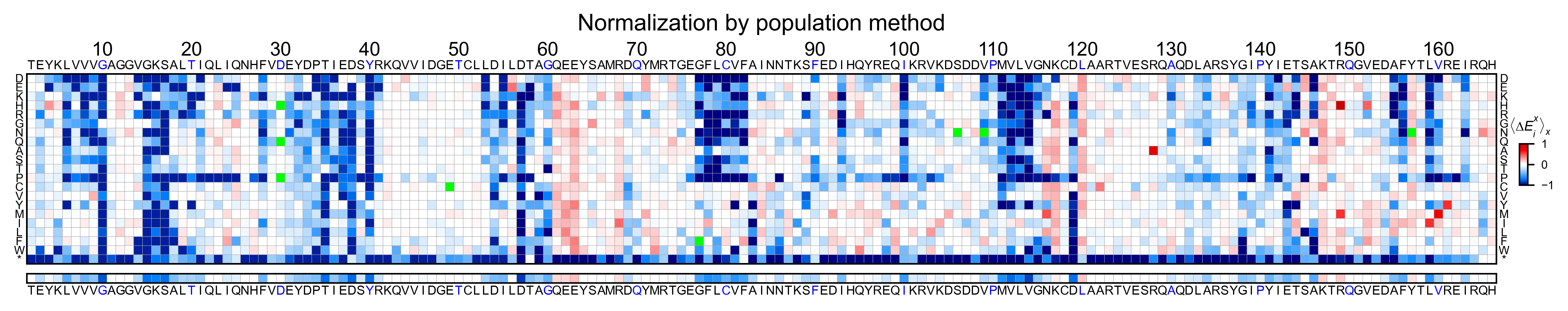
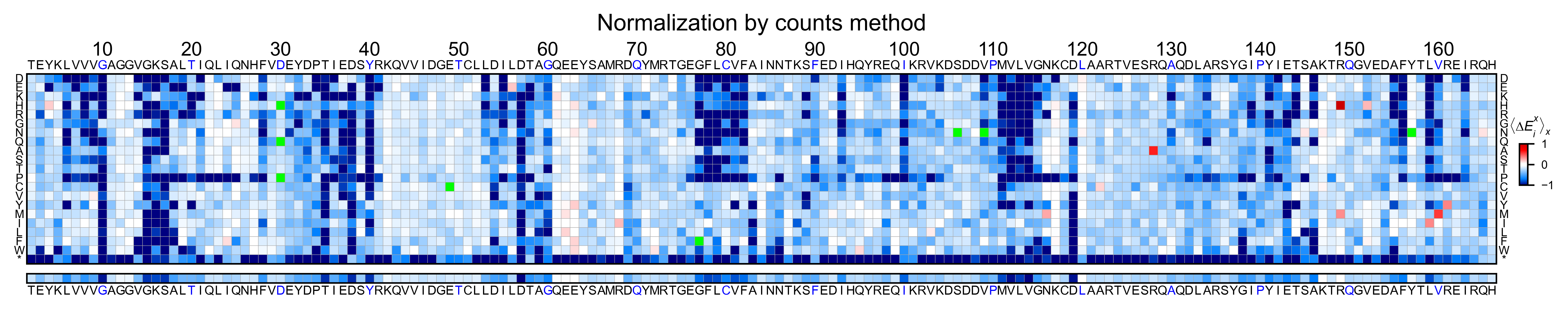
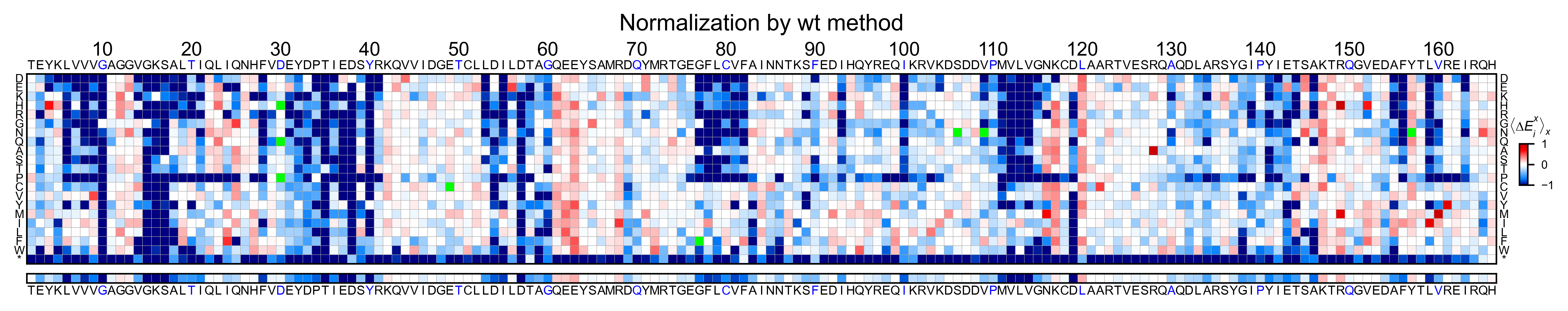
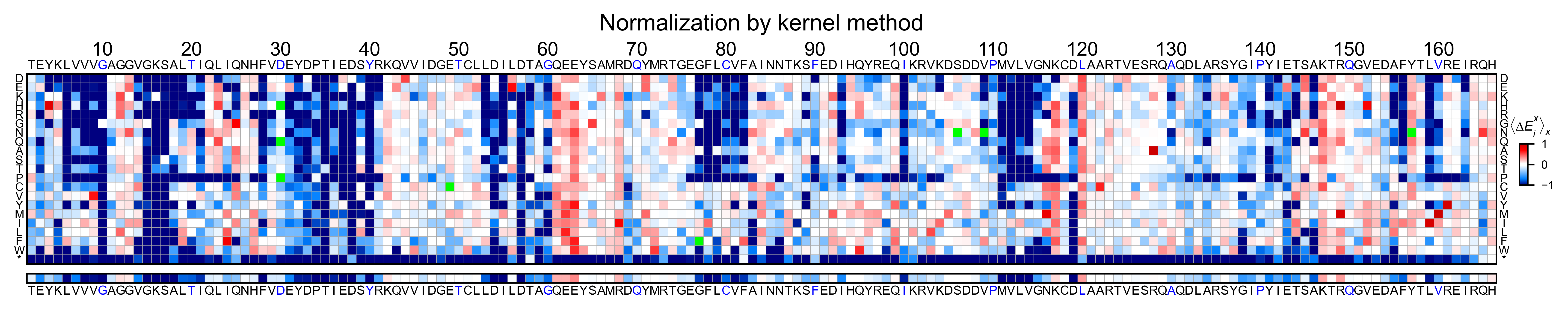
Now that the objects are created and stored in a dictionary, we will use
the method object.heatmap. You will note that the first heatmap
(“population”) looks a bit washed out. If you look at the kernel
distribution, the spread is smaller. The “kernel” and “wt” heatmaps look
almost identical, while the “counts” heatmap looks all blue. This is
caused by the algorithm not being able to center the data properly, and
everything seems to be loss of function. That is why it is important to
select the method of normalization that works with your data.
titles: List[str] = ['population', 'counts', 'wt', 'kernel']

# Create objects
for obj, title in zip(objects.values(), titles):
    obj.heatmap(title='Normalization by ' + title + ' method')