Creating heatmaps
This section shows how to use the mutagenesis_visualization package. The plotting functions can be used regardless of how you process your data. For the examples, we are using two datasets that are derived from Pradeep’s legacy. [1]
Import modules
# running locally, if you pip install then you just have to import the module
%matplotlib inline
from typing import List
import numpy as np
import matplotlib as plt
import copy
from mutagenesis_visualization import Screen
from mutagenesis_visualization.main.utils.data_paths import HRAS_RBD_COUNTS_CSV, HRAS_GAPGEF_COUNTS_CSV
Create object of class Screen
- Class reviewed in this section:
mutagenesis_visualization.main.classes.screen.Screen
In order to create plots, the first step is to create a
Screen.object. The enrichment scores will be passed using the
parameter dataset . The protein sequence sequence and the amino
acid substitutions order aminoacids need to be defined for the
object to be created. Adding the secondary structure secondary is
optional, but without it some plots will not work. In this example, we
are importing two datasets and creating two objects named
hras_GAPGEF and hras_RBD.
# Load enrichment scores. This is how you would load them from a local file.
hras_enrichment_GAPGEF = np.genfromtxt(HRAS_GAPGEF_COUNTS_CSV, delimiter=',')
hras_enrichment_RBD = np.genfromtxt(HRAS_RBD_COUNTS_CSV, delimiter=',')

# Define protein sequence
hras_sequence: str = 'MTEYKLVVVGAGGVGKSALTIQLIQNHFVDEYDPTIEDSYRKQVVIDGETCLLDILDTAGQEEY'\
                + 'SAMRDQYMRTGEGFLCVFAINNTKSFEDIHQYREQIKRVKDSDDVPMVLVGNKCDLAARTVES'\
                + 'RQAQDLARSYGIPYIETSAKTRQGVEDAFYTLVREIRQHKLRKLNPPDESGPG'

# Order of amino acid substitutions in the hras_enrichment dataset
aminoacids: List[str] = list('ACDEFGHIKLMNPQRSTVWY*')

# First residue of the hras_enrichment dataset. Because 1-Met was not mutated, the dataset starts at residue 2
start_position: int = 2

# Define secondary structure
secondary = [['L0'], ['β1'] * (9 - 1), ['L1'] * (15 - 9), ['α1'] * (25 - 15),
             ['L2'] * (36 - 25), ['β2'] * (46 - 36), ['L3'] * (48 - 46),
             ['β3'] * (58 - 48), ['L4'] * (64 - 58), ['α2'] * (74 - 64),
             ['L5'] * (76 - 74), ['β4'] * (83 - 76), ['L6'] * (86 - 83),
             ['α3'] * (103 - 86), ['L7'] * (110 - 103), ['β5'] * (116 - 110),
             ['L8'] * (126 - 116), ['α4'] * (137 - 126), ['L9'] * (140 - 137),
             ['β6'] * (143 - 140), ['L10'] * (151 - 143), ['α5'] * (172 - 151),
             ['L11'] * (190 - 172)]

# Substitute Nan values with 0
fillna: int = 0

# Create objects
hras_GAPGEF: Screen = Screen(
    hras_enrichment_GAPGEF, hras_sequence, aminoacids, start_position, fillna,
    secondary
)
hras_RBD: Screen = Screen(
    hras_enrichment_RBD, hras_sequence, aminoacids, start_position, fillna,
    secondary
)
Heatmaps
- Methods reviewed in this section:
mutagenesis_visualization.main.heatmaps.heatmap.Heatmap()mutagenesis_visualization.main.heatmaps.heatmap_rows.HeatmapRows()mutagenesis_visualization.main.heatmaps.heatmap.columns.HeatmapColumns()mutagenesis_visualization.main.heatmaps.miniheatmap.Miniheatmap()
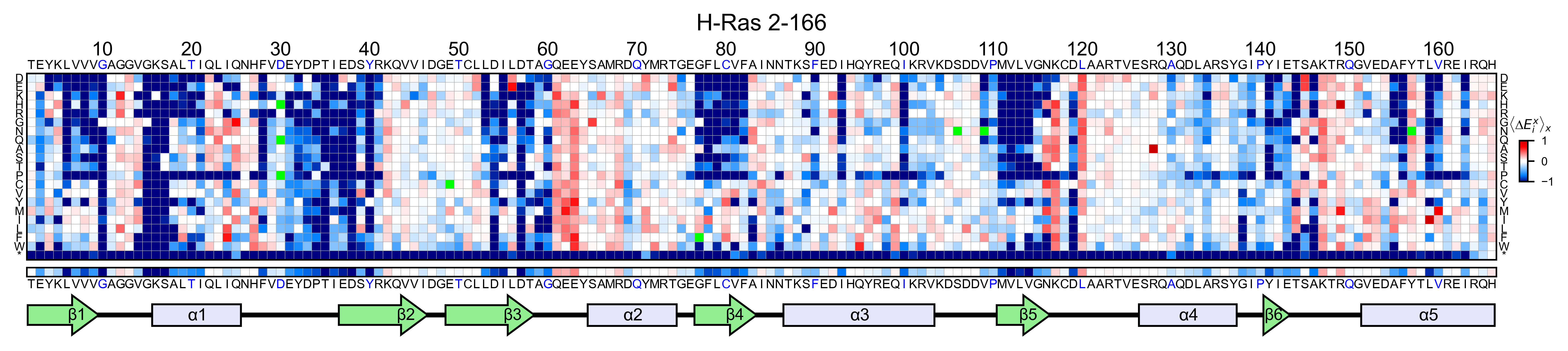
Once the object hras_RBD is created, we will plot a heatmap of the
enrichment scores using the method object.heatmap.
# Create full heatmap
hras_RBD.heatmap(title='H-Ras 2-166', show_cartoon=True)
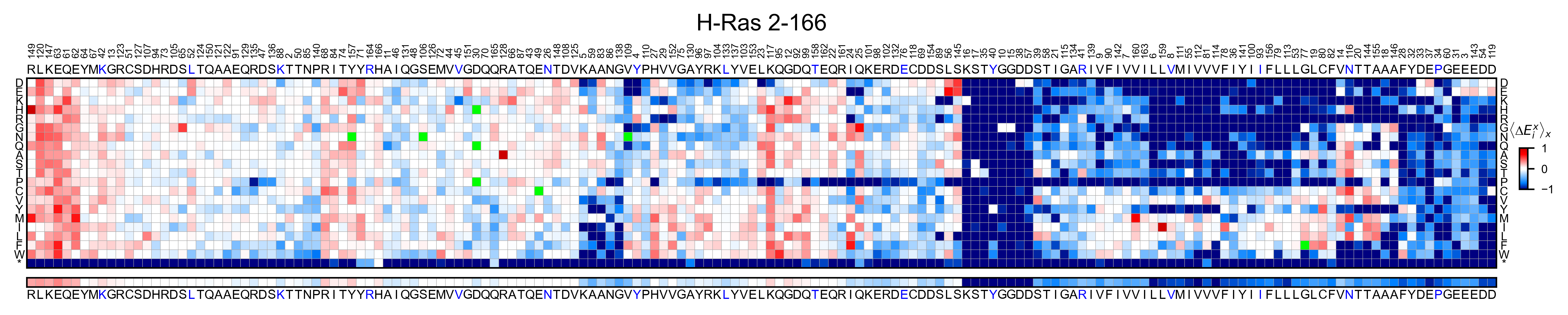
If you set the parameter hierarchical=True, it will sort the columns
using hierarchical clustering
hras_RBD.heatmap(title='H-Ras 2-166', hierarchical=True, output_file=None)
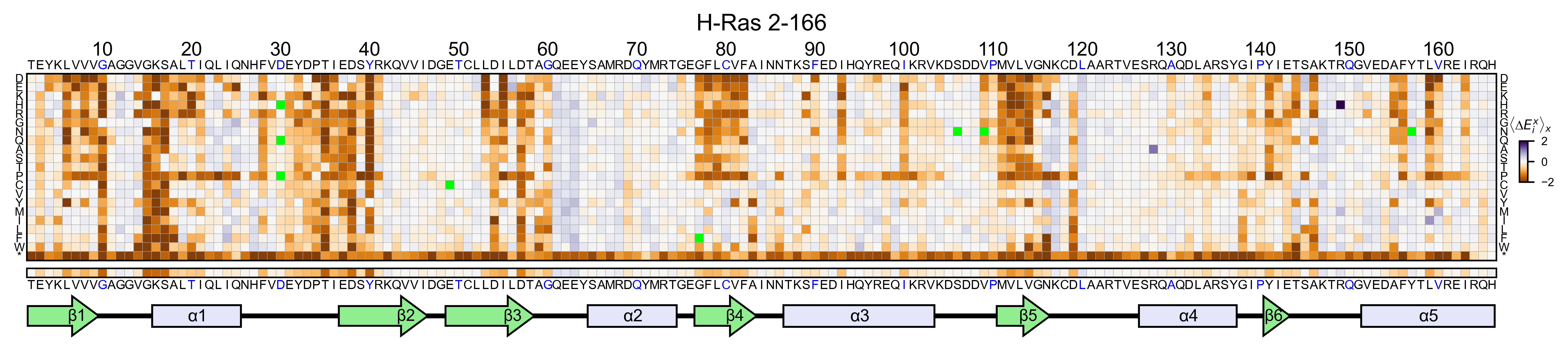
You can change the scale and the color map using the parameters
colorbar_scale and colormap. You can also mask
self-substitutions (ie T2T) by setting mask_selfsubstitutions=True.
The noise in the assay may cause self-substitutions to have a score
different than 0, which may confuse the reader. If you use this masking,
please make sure that there is no systematic error related to the
centering of the data.
# Load a color map from matplotlib
colormap = copy.copy((plt.cm.get_cmap('PuOr')))

# Change scale and colormap
hras_RBD.heatmap(
    mask_selfsubstitutions=True,
    title='H-Ras 2-166',
    colorbar_scale=(-2, 2),
    colormap=colormap,
    show_cartoon=True,
)
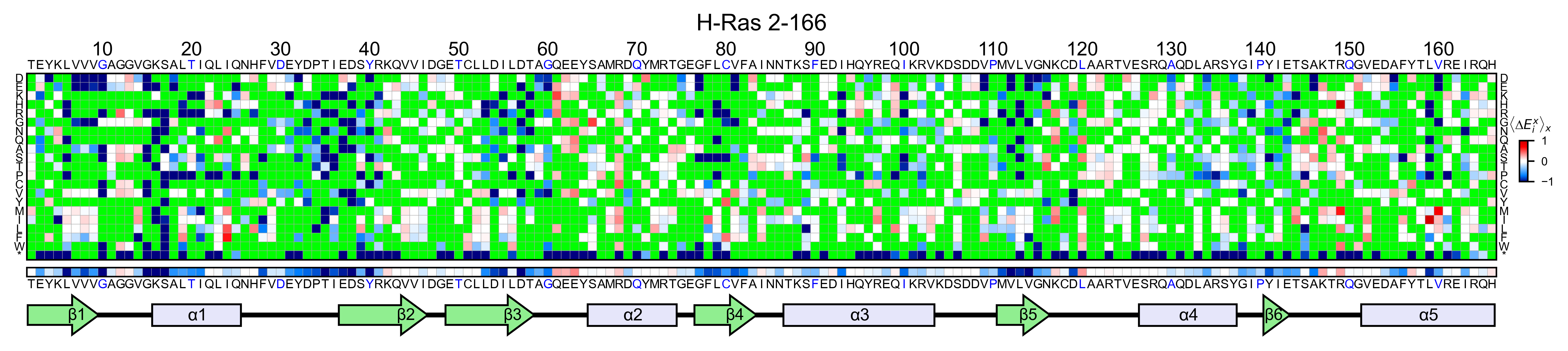
If you set the parameter show_snv=True, the algorithm will color
green every mutation that is not a single nucleotide variant (SNV) of
the wild-type protein. You will notice how many mutations are not
accessible through a nucleotide change. This option may be useful to you
so you can quickly evaluate which mutations are accessible through
random DNA mutations. In the example of Ras, the frequency of non-SNV
substitutions at residues 12 and 13 is dramatically lower.
# Create full heatmap showing only SNV mutants
hras_RBD.heatmap(
    title='H-Ras 2-166', show_cartoon=True, show_snv=True)
We can slice the full heatmap by either showing only some columns or
some rows. To show only a few amino acid mutational profiles (rows), we
will use the method object.heatmap_rows. Note that we need to
specify which amino acids to show with selection.
Heatmap slices
# Create heatmap of selected aminoacid substitutions
hras_RBD.heatmap_rows(
    title='H-Ras 2-166',
    selection=['E', 'Q', 'A', 'P', 'V', 'Y'],
)

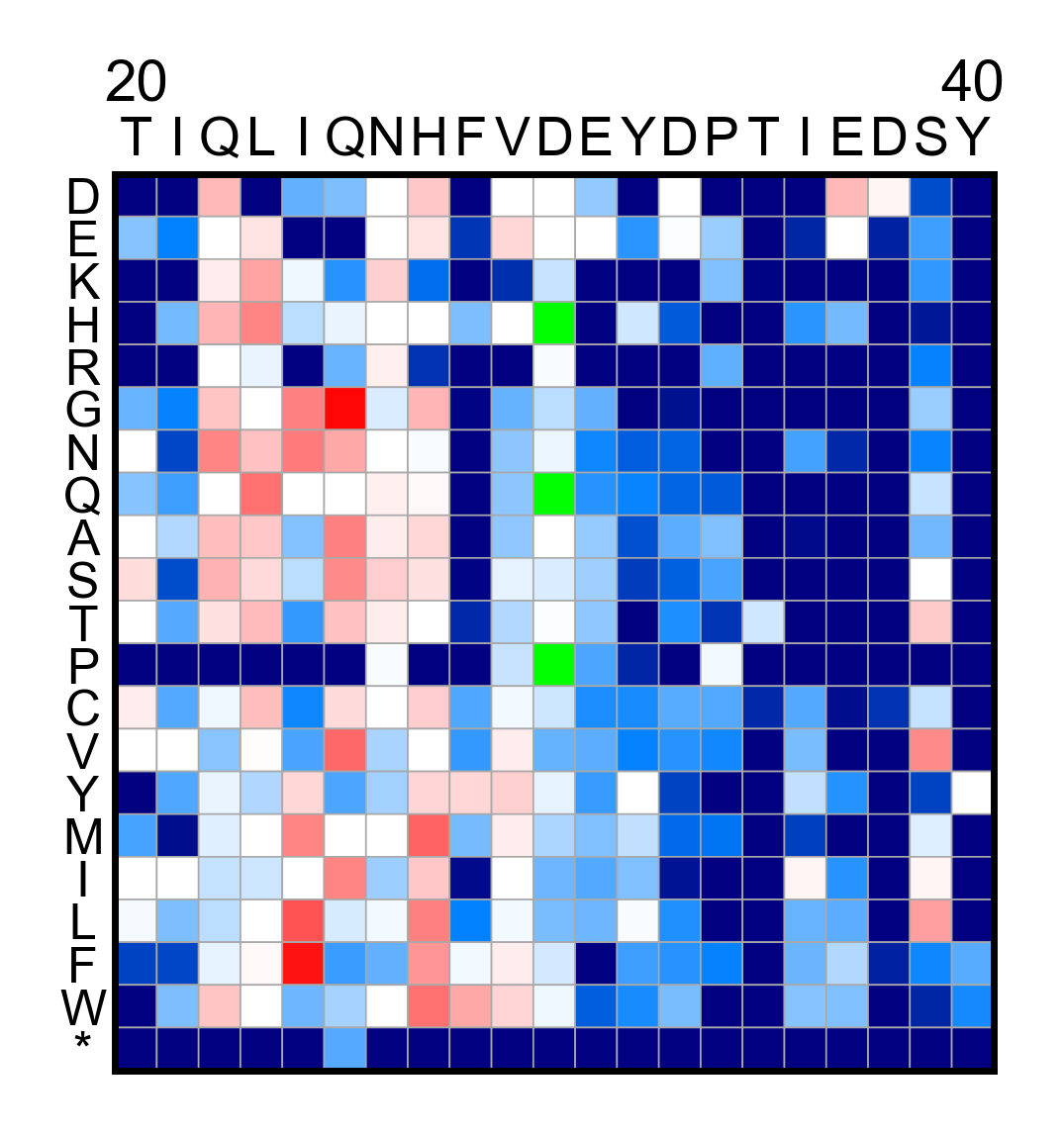
If we want to display only a few positions in the protein (columns), we
will use the method object.heatmap_columns. The parameter
segment will indicate which are the contigous columns to show.
# Create a heatmap of a subset region in the protein
hras_RBD.heatmap_columns(segment=[20, 40])
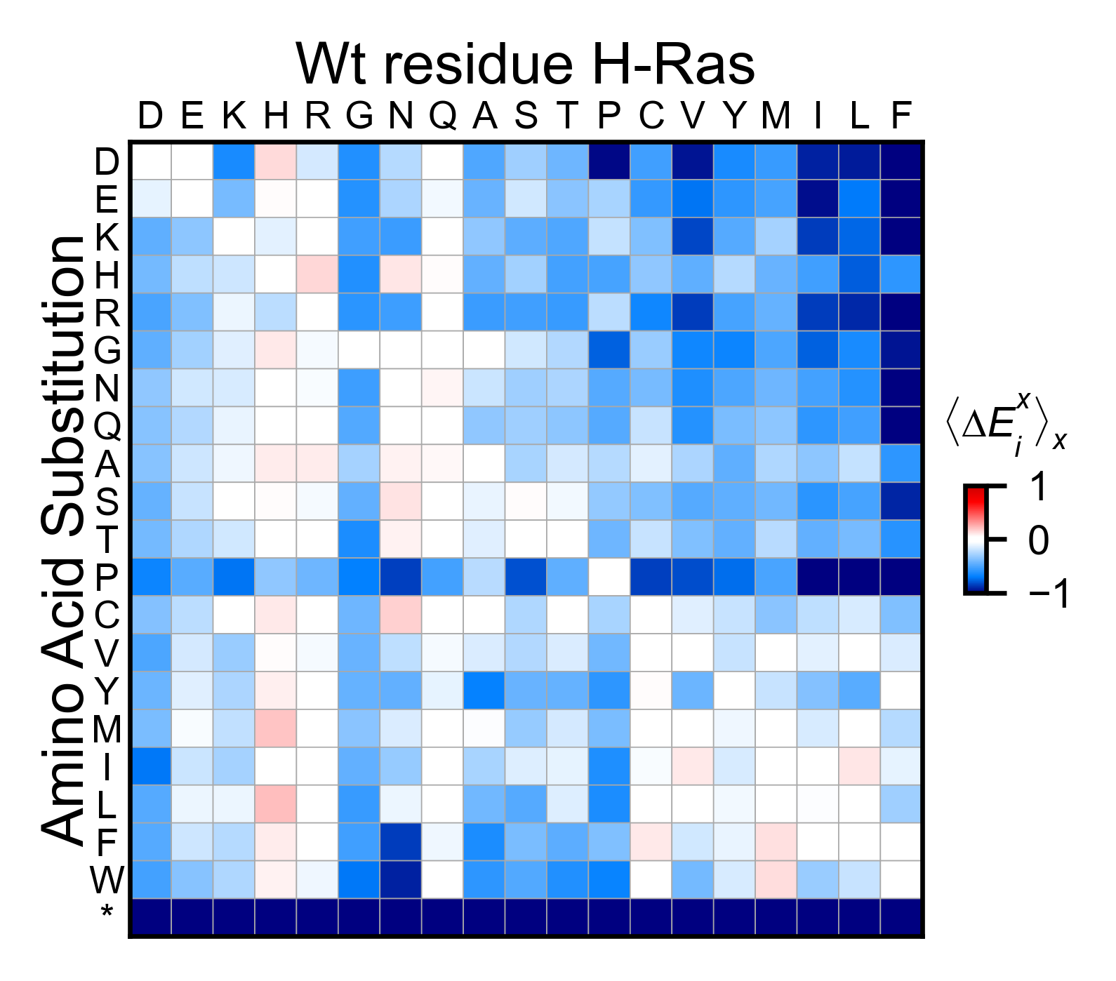
Miniheamap
A summarized heatmap can also be generated. It is useful to evaluate
global trends in the data. The command to use is object.miniheatmap.
# Condensed heatmap
hras_RBD.miniheatmap(title='Wt residue H-Ras')
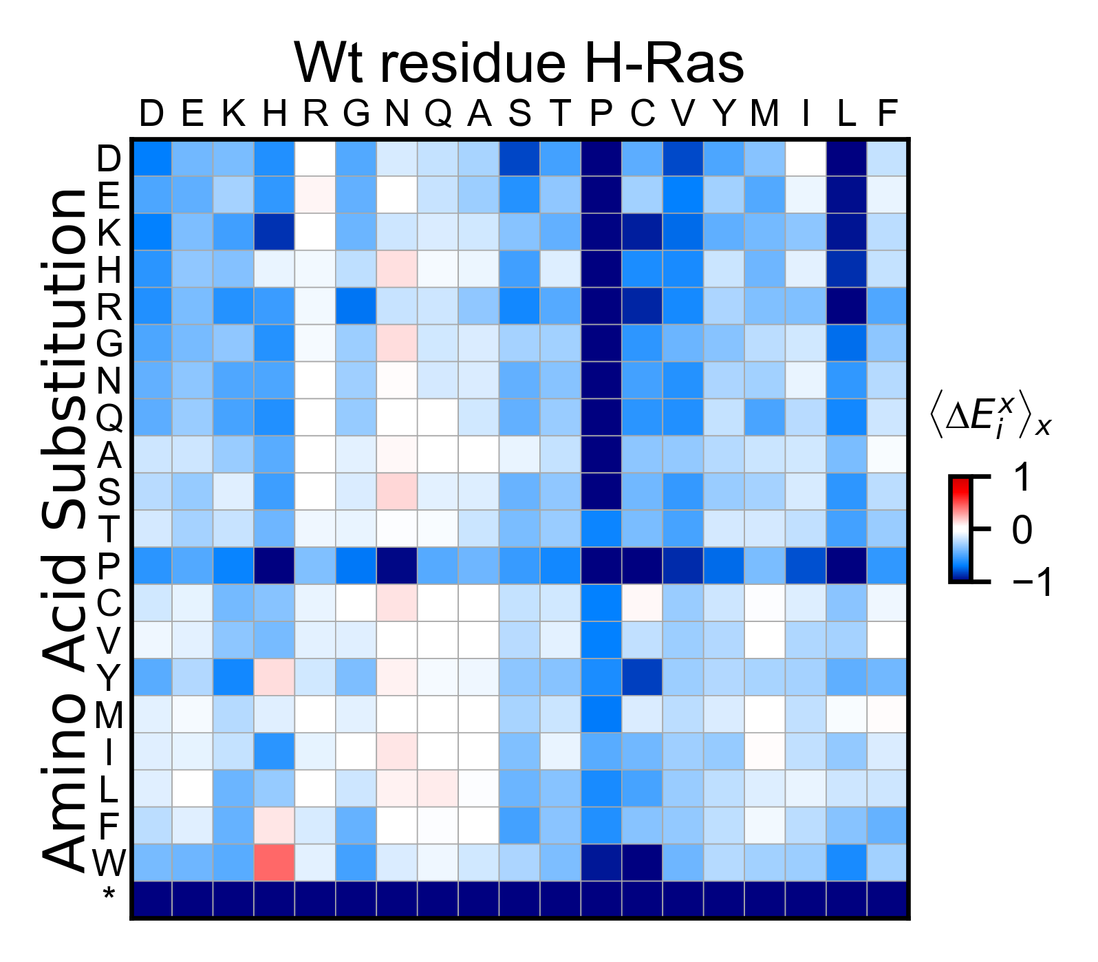
Now lets look at the effect of having a certain residue in front the
mutated residue. For instance, the column of prolines is the average of
all the columns that had a proline in the n-1 position. To accomplish
this, set offset=-1.
# Condensed heatmap offset no background correction
hras_RBD.miniheatmap(
    title='Wt residue H-Ras',
    offset=-1,
    background_correction=False,
)
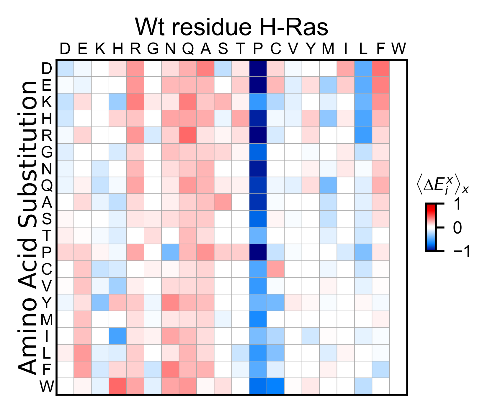
Now lets do a background correction by setting
background_correction=True. To the calculated values, it will
subtract the mean enrichment score for every substitution type. In the
example, proline is the only residues than wen situated before the
mutation, it seems to have a detrimental effect.
# Condensed heatmap offset with background correction
hras_RBD.miniheatmap(
    title='Wt residue H-Ras',
    offset=-1,
    background_correction=True,
)
Reference
| [1] | Bandaru, P., Shah, N. H., Bhattacharyya, M., Barton, J. P., Kondo, Y., Cofsky, J. C., … Kuriyan, J. (2017). Deconstruction of the Ras switching cycle through saturation mutagenesis. ELife, 6. DOI: 10.7554/eLife.27810 |